


Abstract
Within the geo-simulation research domain, micro-simulation and agent-based modeling often require the creation of synthetic populations. Creating such data is a time-consuming task and often lacks social networks, which are crucial for studying human interactions (e.g., disease spread, disaster response) while at the same time impacting decision-making. We address these challenges by introducing a Python based method that uses the open data including that from 2020 U.S. Census data to generate a large-scale realistic geographically explicit synthetic population for America’s 50 states and Washington D.C. along with the stylized social networks (e.g., home, work and schools). The resulting synthetic population can be utilized within various geo-simulation approaches (e.g., agent-based modeling), exploring the emergence of complex phenomena through human interactions and further fostering the study of urban digital twins.
Background & Summary
Within the geo-simulation research domain (e.g., micro-simulation and agent-based modeling) often require the generation of synthetic populations. These synthetic populations have been used to study a plethora of topics within urban systems, such as human mobility, public health, and disaster resilience1,2,3. Researchers such as4 have emphasized the role of geographically- explicit synthetic population in geo-simulation and have created the workflow to nest individuals into different spatial settings (e.g., home, school and workplace). Over time, modelers have also realized that social networks play an important role in human activities as they drive the interactions and lead to aggregate patterns emerging especially in the case of agent-based modeling5,6,7. Over time, researchers have also realized the importance of incorporating social networks as additional layers in the GIS systems8,9,10. By representing people’s relationships using nodes and edges, social networks are suitable to capture complex human interactions (e.g., communication, information sharing and opinion dynamics)8. Integrating social networks into geo-simulation allows researchers to better understand how individuals’ interactions give rise to the emergence of non-linear patterns at a large scale during different circumstances such as green space usage, social segregation and disaster response2,11,12. In our study, we define three types of social networks, home, work and educational as we would argue these can capture most daily interactions13. As modelers, we often spend a significant amount of time creating synthetic populations especially those grounded with data, due to the time needed to collect, preprocess and generate the final synthetic population. Moreover, synthetic populations are often built for a specific purpose which limits their use in other situations. Our aim of this paper is to build and provide a geographically explicit synthetic population along with its social networks using open data including that from the latest U.S. Census which can be used in a variety of geo-simulation models.
Over the last several years, there have been numerous efforts to create synthetic populations (see14 for a review), however, many of these synthetic populations seldom include social networks. Currently, there are several national-level synthetic population datasets, e.g.15,16,17. For example16, the author created a synthetic population for the whole of the US based on 2010 data at the census block level (roughly equivalent to 600 to 3,000 persons) and included various demographic information (e.g., housing type, age, sex, race, and ethnicity). While from a recent work, the authors built a synthetic population for the whole of Canada based on 2016 data and projected out to 2042 using the Canadian dissemination areas (roughly equivalent to 400 to 700 persons)17. In their work both demographic and socio-economic variables (e.g., educational background and income status) where included as agent attributes. Even though these two examples create synthetic populations they present data at an areal unit and do not assign individuals to specific locations, nor do they assign individuals to specific workplaces. At a more local level, efforts have been made to assign home and work locations e.g.4, but social networks are still missing. In what we present below, we not only provide the code and the resulting data but also provide an explicit geographical location (i.e., latitude and longitude) for both home and work locations and include basic social networks. By doing so we provide a way to enable the exploration of basic patterns of life.
When it comes to creating synthetic populations, several methods exist. Each method has its strengths and weaknesses when generating a synthetic population14. Generally speaking, traditional population synthesis methods can be broken into two main approaches: 1) synthetic reconstruction (SR) such as Hierarchical sampling (HS) and Iterative Proportional Fitting (IPF); 2) combinatorial optimization (CO) or re-weighting such as Fitness computation procedures. Many approaches require micro-level data especially those using CO or IPF (e.g., Public Use Microdata Areas (PUMAs) in the US or Samples of Anonymized Records (SAR) in the UK) to calibrate the synthetic populations, e.g.15,17. Additionally, such approaches are computationally expensive and require micro-level data which might not always be available. While HS is a flexible method that does not require such data as input and it only requires data at the aggregated level (e.g., census tract level)18,19. Specifically, HS creates synthetic individuals in a specific order, based on the discrete attributes from the aggregated level data that describe individuals’ characteristics (e.g., males aged from 0 to 4, which are then grouped into a household with married couples and kids). Other than demographic information, our population will have attributes related to work or educational locations along with their explicit geographical locations. Adding these attributes requires our method to handle data from multiple formats (e.g., shapefiles), which needs additional computational resources. Thus, in this work, we utilize HS to generate demographic information due to its flexibility of implementation (e.g., less input data and computational efficiencies). In what follows, we will introduce our method, then present the basic information of the resulting dataset such as data structure, data formats and demonstration of sample data along with the efforts to validate our methodology. The last section will conclude this paper and discuss areas of applications of this dataset.
Methods
Overview
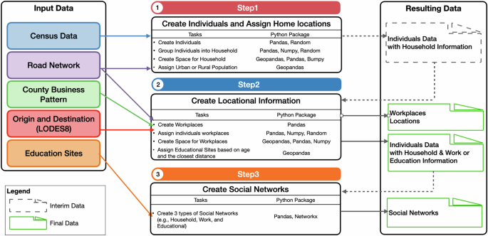
As discussed above, our aim is to generate geographically explicit synthetic population dataset along with their social networks for all 308,745,538 individuals in the United States (i.e., 50 states and Washington D.C.) in 2020. Each individual is assigned a latitude and longitude along with demographic characteristics of gender, age, household information, household structure, work or educational information, which is stored in the GeoPackage (i.e.,.gpkg) format. Additionally, the workplace information (i.e., Workplace ID, latitude and longitude) is also stored using GeoPackage formats. As for the education facilities (i.e., daycares and schools), we use shapefile (i.e.,.shp) to store their unique IDs, latitude and longitude. The social network datasets are stored in comma-separated values (i.e.,.csv) format. Figure 1 shows the workflow of the synthetic generation processes and the following describes it in more detail.

Data Generation Workflow and Resulting Datasets.
Data collection and preprocessing
Due to this work generating the whole U.S. Synthetic population, we created various Python scripts to collect and preprocess data on a state by state basis. Table 1 shows all data collected and utilized in this work along with their data sources. All data for the demographics and workplaces are from the latest 2020 Census Data. While information about educational sites comes from 2015 which is the last time the data was updated20. Data preprocessing included data cleaning (e.g., removing duplicate and null records) from all data, integrating various data (e.g., census data, count business pattern and Origin-Destination Employment Statistics data) into the census tract boundaries, simplifying the road network topology to minimize its size while ensuring all road segments are connected and removing duplicate records from the network (i.e., road segments), while for the education sites data, a unique identifier was added to each location.
Step1: Create individuals and assign home locations
Within Step 1 which is shown in Fig. 1, there are four tasks: (1) creating individuals based on the 2020 US Census data; (2) grouping them into households; (3) placing each household generated in tasks 1 and 2 on residential roads; (4) identifying urban and rural population. As mentioned above, we utilized the Hierarchical sampling (HS) from the Synthetic Reconstruction (SR) method to generate the individuals18. During the generation process, we created individuals within every census tract using gender and age group information extracted from the 2020 US Census data21. The method creates the exact number of individuals by iterating over the 18 age groups for both males and females, such as aged 0 to 4; to 85 and older for males. By doing so, we created individuals whose demographic information such as age and gender can match the U.S. Census’s distribution21.
To group the generated individuals into households, we first created a set of empty household containers of 12 types for each census tract based on the definitions from the US census21. Then, we randomly assign individuals into households to match their household types and conditions. Table 2 shows these household types and the conditions and assumptions used to place individuals while ensuring they fit the characteristics expected for each household type. As for group quarters (which in the US refer to places like college residence halls, aging facilities and correctional institutions), the exact number of the population is assigned into group quarters. Since we do not have information about the number of group quarters, we aggregate all group quarters in a census tract into one household and assign them a unique identifier. These assumptions on assignments can be refined if readers so desire, this is one reason we provide the code to generate the synthetic population.
Once the households have been created, we then give them a home location by using the road networks as a proxy for actual buildings. Our rationale for this is that assigning individuals/households a home location allows modelers to incorporate the ability to add movement to agents and thus the ability to explore a wide range of issues (e.g., urban mobility, commuting activities, transportation). Meanwhile, using street networks rather than building footprints can preserve a certain level of privacy. Thus, the home location is extracted from the road network, specifically, we identified all residential roads within a tract and placed each household along these roads. We randomly assign individuals to any residential road and attempt to keep them 50 meters apart to distribute them evenly throughout the census tract. However, when this is not possible, household locations will be placed on top of each other (like in dense urban areas). An example of this is shown in Fig. 2. Additionally, we assign individuals with urban or rural attributes based on where they have been assigned utilizing US census definitions22. At the end of this step, each generated synthetic individual will have a unique ID along with basic demographics such as age, gender, household type, household ID, home location, and urban or rural tag.

Examples of Generated Household Locations in Census tracts that are (a) Suburban and (b) a High-Density Urban.
Step2: Create locational information
As shown in Fig. 1, four tasks related to individuals’ daytime locational information are constructed in Step 2: (1) creating workplaces with unique IDs; (2) assigning workplace to work population; (3) placing each workplace generated in Tasks 1 along the roads; (4) assigning educational sites to children. The workplace information is based on the County Business Patterns data23 and Longitudinal Employer-Household Dynamics (LEHD) Origin-Destination Employment Statistics (LODES 8)24 from the 2020 Census. Additionally, using LODES 8, we can extract the number of the employed population. Then, we assign individuals created in Step 1 with a workplace as their daytime location. For individuals not assigned a workplace, their daytime locations will be their household locations.
To assign each workplace a geographical location, we place the workplaces on the secondary roads 20 meters apart and the intersections of secondary and residential roads. the secondary road refers to the main road without limited access, including U.S. highway, state highway, or county highway systems25. Furthermore, we assigned children (aged 0 to 17) to the closest daycare/schools based on their ages (e.g., daycare, elementary, middle, and high school) whose locations were sourced from the US Environmental Protection Agency (EPA) Office of Environmental Information (OEI)20. The assumptions used to assign children to educational sites are as follows: ages 0–4 to Daycare, ages 5–11 to Elementary School, ages 12–14 to Middle School, and ages 15–17 to High School, which could also be refined based on different modeling circumstances.
Step3: Create social networks
Lastly, as mentioned above, social networks are included in our synthetic population. Three types of social networks are created based on (1) being in the same household, (2) working in the same workplace, or (3) attending the same educational site. Small-world networks26 are created for people whose household, workplace or education site has more than 5 people, where the number 5 is chosen to indicate the size of the core social group with 5 people based on the work of Dunbar27, where the size of an individual’s educational and work networks ranged from a minimum of 0 to the maximum of 14. While for people in the same household, workplace or education site with 5 or less than 5 people, everyone is fully connected. Within this step, we use the Python package called networkx to create such social networks with its built-in function “newman_watts_strogatz_graph(n, k, p)”. The n indicates the total number of the population (i.e., nodes). To mimic the core social group of 5 people, we should set up the following parameters, specifically, the k is 4, which means one person can be connected to 4 people to make up a 5 people social group, the p is set as 0.3, which indicates the probability of adding a new edge between non-adjacent nodes, to enable us to have a variation on edges, where indicates some of them have more or less connection. It should be noted that unlike the other networks, the work network was generated at the national level due to people working across state boundaries and then partitioned at the state level.
Data Records
The dataset is available at OSF28. Interested readers can download the geographically explicit synthetic population along with their social networks by state. After the generation process, we have generated 330,526,186 individuals for America’s 50 states and Washington D.C., where each has six resulting datasets. Table 3 shows the basic information of the resulting datasets such as data format and detailed descriptions. Tables 4, 5 shows the description of the variables from the generated synthetic population and workplace datasets. Each individual has a set of geographical locations that represent their home, work or school addresses. Additionally, these individuals are not isolated, they are embedded in a larger social setting based on their household, working and studying relationships. As for the social network datasets, each row represents a social network. The index 0 of each row is the starting node, the rest n of the row is a set of neighbors of the social network, where n differs in size depending on the network, n ∈ [0, 14]). To show how our synthetic networks can be related to geographically explicit locations, Fig. 3 shows a selected synthetic household’s geographic location and its member’s workplace, school and daycare locations, where the zoomed-in figure lays out the selected household’s social networks (i.e., educational, work and household). Figure 4 shows our four sample networks extracted from the City of Buffalo in New York State while the resulting networks averaged properties at the national-level are presented in Table 6.

A Sample of a Social Networks for one Household and their Home, Work and Educational Social Networks from the Generated Data.

Sample of Generated Social Networks Extracted from the City of Buffalo, New York: (a) Household; (b) Work; (c) School; (d) Daycare.
Technical Validation
In this work, we first conducted internal validation to ensure that our resulting synthetic population aligns with the input census data at multiple levels (i.e., individual, household and census tract). As for the individual level, other than checking if the number of synthetic individuals matches the census records by reporting the total absolute error (TAE) and Absolute Percentage Difference (APD), we also ensured the male and female populations under the different 18 age groups matched with the U.S. Census data. We compared the number of individuals in our synthetic population and Census under each age group using APD. Similar procedures are conducted at the household level, we compared the total synthetic household number to census records using APD. Additionally, at the census tract level, we compared the household size of synthetic and census data by reporting TAE. TAE and APD are commonly used error metrics for the quality check and validation of generated synthetic population14,18.
During the synthesis process, we found some census tracts had errors. The majority of these problematic tracts are located in parks or nature reserves, which had inconsistent counts with respect to total numbers of males and females or no data was given from the official US Census data. Thus, we can not generate a synthetic population for those problematic tracts and we only input the census tracts excluding the problematic tracts (i.e., Good Census Tracts) to generate the synthetic population. In total, there were 428 problematic tracts which only represent 0.51% of all census tracts. Table 7 shows the TAE on population between All Census Tracts (i.e., 83,848 tracts) and Good Census Tracts (i.e., 83,420 tracts), which indicates the population living in problematic tracts is only 0.279% compared to the whole U.S. (50 states and D.C.) population. In addition, the matching number on the total number of synthetic population and the population living in Good Census Tracts shows that our method can generate the exact number of population from the input census tracts. As for the total household numbers, we generate 126,442,118 households which when compared to Good Census Tracts is 5,601 less, but the difference is only 0.004% as shown in Table 7. This could be due to how we handle group quarters or household assignments (e.g., Table 2).
As our method generates the synthetic population and assigns them into households based on the household type, we also compared both the male and female population for different age groups and households (excluding group quarter households) from the synthetic data with the Good Census and All Census Tracts to report APD. As our method generates the identical number under each age group as the Good Census Tracts, the APD for both males and females are all zero. When comparing synthetic data to All Census Tracts, the male’s average APD is 0.3% and for female is 0.2%. With respect to the comparison on household types’, when compared to All Census Tracts, the average APD is 0.3%. While comparing to the Good Census Tracts, the average APD is 0.02%. It should be noted that these low APDs indicate that our generated synthetic population has very minor differences when compared to the input census data as shown in Fig. 5.

Validation of the Synthetic Population at Different Levels: (a) Population under Different 18 Age Groups; (b) Household under Different Household Types.
Turning to average household size, based on the 2020 American Community Survey (ACS), the overall estimated average household size was 2.6 with a margin of error ±0.0129. As Table 7 shows, the average household size from the 2020 Census Data and our synthetic population is 2.61, which is the same as the ACS data. In addition, we also compare the average household size at the census tract level with our synthetic data and calculate the average household size using the tract’s total population divided by the tract’s total number of households. Figure 6 shows the comparison on the average household size between our synthetic population and census data. Each blue dot represents a census tract. If the blue dots overlap with the red line (i.e., the line of equality), it indicates no difference between our synthetic population data and census data regarding the average household size for that specific tract. If the blue dots are above the red line, the average household size in our synthetic data is larger. Conversely, if the blue dots are below the red line, the average household size in our synthetic data is smaller. The closer the dots are to the red line, the smaller the differences areTo better show the distribution of the differences, we use the ln for both the x and y axes. Out of the total of 83,420 census tracts, our method generated 32,231 tracts’ population with the same average household size and 82,968 tracts’ where the average household sizes have absolute differences of less than 0.1. One potential reason for this is that we consider group quarters as households in our method (see Step 1 in the Methodology Section). Which in turn means that in some tracts with universities for example, there might be 5000 people who are grouped into one household. This increases the average household size potentially when scaling to the whole of the US.

Validation of Average Household Size: Synthetic Population and Census Data on a Logarithmic Scale (ln) where each blue dot represents a census tract.
After comparing our synthetic population to the input census data (i.e., in tract level), we also conducted two external validation experiments by utilizing the American Community Survey Public Use Microdata Sample (ACS PUMS) and the census data at the block group level. As for the first external validation experiment, we compared our synthetic population to ACS PUMS, which contains a sample of five percent of individuals who have been surveyed and recorded in the census. Each individual from ACS PUMS has the same attributes of age and gender as our resulting synthetic population. Thus, we can check if the male and female populations under the different age groups from the ACS PUMS and our resulting synthetic population share similar distributions. In this process, we collected 2022 ACS PUMS data30, because this is the only data that uses the latest 2020 Public Use Microdata Areas (PUMA) as the geographical boundaries. Each PUMA contains several census tracts from the latest 2020 census, which allows us to aggregate our resulting synthetic population into PUMAs. While the 2020 and 2021 ACS PUMS use 2010 PUMAs and it’s not possible to conduct the same aggregation with 2020 and 2021 ACS PUMS. Following the same approach presented by16’s external validation of calculating cosine similarity for each PUMAs, we aggregate the resulting synthetic population and 2022 ACS PUMS into 2462 PUMAs to make comparisons. The cosine similarity ranges from −1 to 1, where a similarity of 1 means the two sets of data are identical. Figure 7 demonstrates the distribution of cosine similarity for the 2462 PUMAs and shows that 96% of PUMAs have a cosine similarity greater than 0.95. This indicates that the resulting synthetic population generated using our method shares a similar age distribution to ACS PUMS.
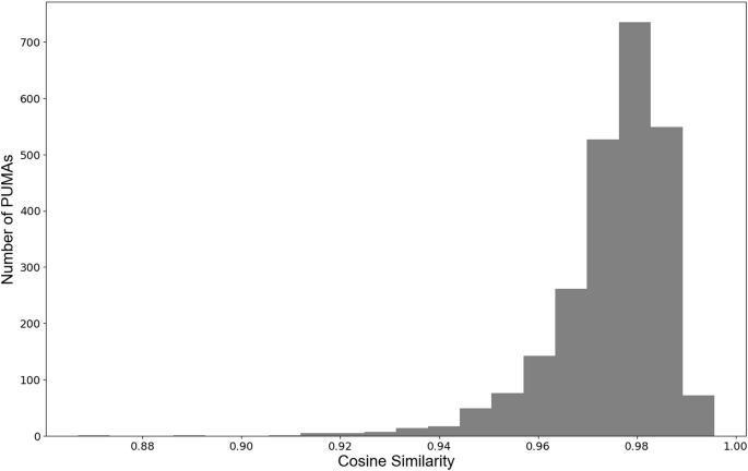
The Distribution of Cosine Similarity between Synthetic Population and the American Community Survey Public Use Microdata Sample (ACS PUMS) for the 2462 Public Use Microdata Areas (PUMA).
Turning to the utilization of block group level’s census data, we have calculated the Spearman’s rank correlation of all census tracts of the whole U.S. Specifically, we have calculated the number of our synthetic population in each census block group by using individuals’ latitude and longitude information, where a census block group is one of the multiple subdivisions of a census tract. Next, for each tract, we calculated the Spearman’s rank correlation between our synthetic population and the real population in its census block groups. A Spearman’s rank correlation value in the range of 0.5 to 1 indicates a near-perfect match (strong positive correlation) when comparing our synthetic population to the census record at the census block group level. As the Table 8 shows, the percentage of tracts with a Spearman’s rank correlation value in the range of 0.5 to 1 are 54% for the whole US. for the whole US. In the sense, our method can capture the population’ spatial distribution on a finer scale to some extent, which indicates our method works better in high population density states, such as New Jersey (NJ) with 59.09%, Rhode Island (RI) 61.13% and Massachusetts (MA) 59.5%. However, one point to be noted is that the initial design of our method did not intend to capture the accurate geographic locations with data (e.g., building footprints) in order to avoid the privacy issues.
To summarise, our method can generate the number of individuals for good census tracts (see Table 7) and the resulting population age distribution aligns to the census records and ACS PUMS. In addition, the Spearman’s rank correlation calculated from the census data from block group level suggests that our method can capture a finer scale of the population’s spatial distribution. Other than these, the method groups individuals into 12 household types (shown in Table 2) and the distribution of the number of households under each type also corresponds with census records. For example, with respect to the average household size, our method can generate ± 99.5 of census tracts with absolute differences of less than 0.1. Thus, our method can generate a baseline synthetic population dataset with stylized social networks.
Usage Notes
The resulting dataset with geographical information can be loaded using GIS software (e.g., ArcGIS), R and Python data management packages (e.g., pandas, geopanadas). To apply these data for geo-simulation modeling purposes, these data can be utilized to initialize microsimulations and agent-based models within various platforms (e.g., MATsim, Netlogo and GAMA) and programming languages (e.g., Pyhton, Java and R). The social network datasets can be loaded and applied using the Python networkx package and Gephi for further analysis and visualization.
Potential use cases for this data, for example, within agent-based modeling, this data could be used to model the emergence of phenomena through individual interactions. These topics could fall into urban planning, e.g.31, transportation, e.g.32, and public health research e.g.2,33. In addition, the method and the data from this work could potentially address the concerns with urban digital twins which often lack demographic, economic, and social processes34, in the sense by providing agents to populate such worlds.
However, as with all work, there is always room for improvement. We would like to point out the use cases where this data might not be applicable. First, because of the nature of the systemic data which is only a snapshot in time (i.e., 2020), the data can not be used directly to study the long-term evolution of the population such as long-term migration and aging populations, however, approaches (e.g., dynamic microsimulation methods) could be further applied on the data to extend this data’s capability to explore such topics e.g.17. Furthermore, the dataset was not designed to account for different modes of transportation (e.g., taking public transportation, carpooling, driving, walking) or for the fine-scale movement of individuals such as building evacuation styles of models. We chose to omit building footprints to avoid potential privacy issues or misrepresentation. However, the method presented here could be extended by incorporating such data (e.g., high- resolution building footprint data or land use data or travel surveys for model of commuting) to guide the geographic location assignments4 and commute type assignments for the synthetic population, which may allow the resulting data to study finer-scale dynamics such as detailed individual-level mobility dynamics, building evacuation. Even with these limitations, the baseline geographically explicit synthetic population and the estimated social networks can be utilized to explore various topics in America’s 50 states and Washington D.C. We look forward to learning how researchers will utilize this data.
Code availability
This work (e.g., data collection, data preprocessing and generation processes) is coded using Python 3.12 and all the scripts used are available at: https://github.com/njiang8/geo-synthetic-pop-usa.
References
-
Ersing, R. L. & Kost, K. A. Surviving Disaster: The Role of Social Networks (Lyceum Books, Chicago, IL, 2012).
-
Yin, F., Crooks, A. & Yin, L. How information propagation in hybrid spaces affects decision-making: using abm to simulate covid-19 vaccine uptake. Int. J. Geogr. Inf. Sci. 38, 1109–1135 (2024).
-
Kim, J. S. et al. Location-based social network data generation based on patterns of life. In 2020 21st IEEE International Conference on Mobile Data Management (MDM), 158–167 (IEEE, 2020).
-
Chapuis, K., Taillandier, P., Renaud, M. & Drogoul, A. Gen*: a generic toolkit to generate spatially explicit synthetic populations. Int. J. Geogr. Inf. Sci. 32, 1194–1210 (2018).
-
Hamill, L. & Gilbert, N. Social circles: A simple structure for agent-based social network models. J. Artif. Soc. Soc. Simul. 12, 3 (2009).
-
Heppenstall, A. et al. Future developments in geographical agent-based models: Challenges and opportunities. Geogr. Analysis 53, 76–91 (2021).
-
Batty, M. The New Science of Cities (MIT press, Cambridge, MA, 2013).
-
Andris, C. Integrating social network data into gisystems. Int. J. Geogr. Inf. Sci. 30, 2009–2031 (2016).
-
Gallagher, K., Anderson, T., Crooks, A. & Züfle, A. Synthetic Geosocial Network Generation. In Proceedings of the 7th ACM SIGSPATIAL Workshop on Location-based Recommendations, Geosocial Networks and Geoadvertising, LocalRec ’23, 15–24 (2023).
-
Züfle, A. et al. In Silico Human Mobility Data Science: Leveraging Massive Simulated Mobility Data (Vision Paper). ACM Trans. Spatial Algorithms Syst. 10, 13:1–13:27 (2024).
-
Li, W., Yuan, J., Ji, C., Wei, S. & Li, Q. Agent-based simulation model for investigating the evolution of social risk in infrastructure projects in china: a social network perspective. Sustain. Cities Soc. 73, 103112 (2021).
-
Sert, E., Bar-Yam, Y. & Morales, A. J. Segregation dynamics with reinforcement learning and agent based modeling. Sci. reports 10, 11771 (2020).
-
Gumber, C. & Burrows, M. Hybrid/Mixed Work Still Unusual, But Increasingly Common in 2021. Report No. P70BR-184 (U.S. Census Bureau, 2023).
-
Chapuis, K., Taillandier, P. & Drogoul, A. Generation of synthetic populations in social simulations: a review of methods and practices. J. Artif. Soc. Soc. Simul. 25 (2022).
-
Wheaton, W. D. et al. Synthesized Population Databases: A US Geospatial Database for Agent-based Models. Report No. MR-0010-0905 (RIT Press, 2009).
-
Lin, Y. Synthetic population data for small area estimation in the United States. Environ. Plan. B: Urban Anal. City Sci. 51, 553–562 (2024).
-
Prédhumeau, M. & Manley, E. A synthetic population for agent-based modelling in Canada. Sci. Data 10, 148 (2023).
-
Barthelemy, J. & Toint, P. L. Synthetic population generation without a sample. Transp. Sci. 47, 266–279 (2013).
-
Wise, S. Using social media content to inform agent-based models for humanitarian crisis response. PhD Dissertation, George Mason University, Fairfax, VA (2014).
-
USEPA. Educational Institutions, US, 2015, ORNL, SEGS. https://edg.epa.gov/metadata/catalog/search/resource/details.page?uuid=%7B9C49AE4B-F175-43D0-BCC6-A928FF54C329%7D (2015).
-
U.S. Census Bureau. Decennial Census 2020 Census Demographic Profile. https://www.census.gov/data/tables/2023/dec/2020-census-demographic-profile.html (2024).
-
U.S. Census Bureau. TIGER/Line®Shapefiles: Urban Areas. https://www.census.gov/cgi-bin/geo/shapefiles/index.php?year=2020&layergroup=Urban+Areas (2020).
-
U.S. Census Bureau. All Sectors: County Business Patterns. https://www2.census.gov/programs-surveys/cbp/data/2020/CB2000CBP.zip (2022).
-
U.S. Census Bureau. LEHD Origin-Destination Employment Statistics (LODES). https://lehd.ces.census.gov/data/lodes/LODES8/?C=D;O=A (2023).
-
U.S. Census Bureau. 2020 TIGER/Line® Shapefiles: Roads. https://www.census.gov/cgi-bin/geo/shapefiles/index.php?year=2020&layergroup=Roads (2020).
-
Watts, D. & Strogatz, S. H. Collective dynamics of ‘small-world’ networks. Nature 393, 440-442 (1998).
-
Dunbar, R. I. M. The social brain hypothesis. Evol. Anthropol. Issues, News, Rev. 6, 178–190 (1998).
-
Jiang, N., Yin, F., Wang, B. & Crooks, A. Large-Scale Geographically Explicit Synthetic Population for the United States. OSF. https://doi.org/10.17605/OSF.IO/FPNC2 (2024).
-
U.S. Census Bureau. American Community Survey. https://data.census.gov/table/ACSST5Y2020.S1101 (2020).
-
U.S. Census Bureau. PUMS Data. https://www2.census.gov/programs-surveys/acs/data/pums/2022/5-Year/ (2023).
-
Heppenstall, A. J., Crooks, A. T., See, L. M. & Batty, M. Agent-based models of geographical systems (Springer, Dordrecht, 2011).
-
Jiang, N., Crooks, A. T., Kavak, H., Burger, A. & Kennedy, W. G. A method to create a synthetic population with social networks for geographically-explicit agent-based models. Comput. Urban Sci. 2, 7 (2022).
-
Bard, J. E. et al. Genomic profiling and spatial SEIR modeling of COVID-19 transmission in Western New York. Front Microbiol. 15, 1416580 (2024)
-
Malleson, N., Franklin, R., Arribas-Bel, D., Cheng, T. & Birkin, M. Digital twins on trial: Can they actually solve wicked societal problems and change the world for better? Environ. Plan. B: Urban Anal. City Sci. 51, 1181–1186 (2024).
-
U.S. Census Bureau. 2020 TIGER/Line® Shapefiles: Census Tracts. https://www.census.gov/cgi-bin/geo/shapefiles/index.php?year=2020&layergroup=Census+Tracts (2020).
Author information
Authors and Affiliations
Contributions
The idea was conceptualized by N.J. and A.T.C.. N.J. and B.W. designed the workflow and experiments and N.J. coded the model and carried out the experiments, which along with F.Y. conducted the analysis and wrote up the results. Both A.T.C. and N.J. prepared the initial draft while F.Y. and B.W. provided substantial edits and suggestions to the paper and all authors approved its content.
Corresponding author
Ethics declarations
Competing interests
The authors declare no competing interests.
Additional information
Publisher’s note Springer Nature remains neutral with regard to jurisdictional claims in published maps and institutional affiliations.
Rights and permissions
Open Access This article is licensed under a Creative Commons Attribution-NonCommercial-NoDerivatives 4.0 International License, which permits any non-commercial use, sharing, distribution and reproduction in any medium or format, as long as you give appropriate credit to the original author(s) and the source, provide a link to the Creative Commons licence, and indicate if you modified the licensed material. You do not have permission under this licence to share adapted material derived from this article or parts of it. The images or other third party material in this article are included in the article’s Creative Commons licence, unless indicated otherwise in a credit line to the material. If material is not included in the article’s Creative Commons licence and your intended use is not permitted by statutory regulation or exceeds the permitted use, you will need to obtain permission directly from the copyright holder. To view a copy of this licence, visit http://creativecommons.org/licenses/by-nc-nd/4.0/.
About this article

Cite this article
Jiang, N., Yin, F., Wang, B. et al. A Large-Scale Geographically Explicit Synthetic Population with Social Networks for the United States.
Sci Data 11, 1204 (2024). https://doi.org/10.1038/s41597-024-03970-1
-
Received:
-
Accepted:
-
Published:
-
DOI: https://doi.org/10.1038/s41597-024-03970-1
This post was originally published on this site be sure to check out more of their content