


Abstract
Grounded in the universal human predisposition to seek social connection, this study uniquely integrates social media data with mobility patterns to provide a holistic view of public emotional dynamics during the pandemic. Drawing on 45 million geocoded tweets from SINA.com, 57 billion trip records across 335 cities from Tencent Location Big Data, and 296 million mutual following records from social media users, we construct a large-scale, daily city-level emotional metric across different stages of pandemic. Our findings reveal significant emotional autocorrelation across different ties and identify four distinct feedback mechanisms shaping emotional interactions during the pandemic: amplified positive feedback in social media ties during the warning phase; shrinking positive feedback in geographic ties during the isolation phase; and negative and asymmetric feedback in social media and mobility ties, respectively, during the normalization phase. Notably, the easing of pandemic restrictions corresponded with a surge in positive emotional interactions in geographic and mobility ties. These findings underscore the role of physical and digital social networks, spanning geographic, mobility, and social media ties, in shaping public emotional interactions throughout different pandemic stages. Understanding these dynamics can inform crisis communication strategies, mitigate public distress, and enhance social resilience, offering valuable insights for policymakers managing future large-scale disruptions.
Introduction
The COVID-19 pandemic, though no longer classified as an emergency of international public health concern, has had far-reaching consequences on public health preparedness and response mechanisms. At the peak of the crisis, global anxiety levels surged dramatically, with studies reporting a 25% increase in the prevalence of anxiety and depression worldwide (World Health Organization, 2022). It is regarded as one of the most severe infectious diseases in history (Perlman 2020), prompting critical scrutiny of emergency response systems. As a result, the pandemic has become a focal point of extensive academic research aimed at understanding its lessons. These lessons are crucial for shaping policy-making, strategic planning, and the implementation of public health interventions, thereby strengthening global resilience against future pandemics (Catania et al. 2021; Logemann et al. 2022; Peeri et al. 2020).
Understanding public sentiment during crises is essential for effective crisis communication, as emotional reactions can influence behavioral responses, compliance with health measures, and overall crisis management (Wise et al. 2020). The public’s negative emotional response to uncertain and risky situations significantly impacts decision-making processes and social behaviors (Rottenstreich and Hsee 2001; Slovic et al. 2013). Consequently, monitoring real-time public emotions becomes a vital component of risk prevention and crisis management (Zhang et al. 2021). While social media has emerged as a valuable tool for tracking public sentiment (Kahneman and Krueger 2006), an effective crisis response requires a more comprehensive understanding of how emotions propagate through social structures, including both physical and digital networks.
The psychological and social consequences of public crises are topics of increasing importance in research, as demonstrated by the wealth of studies that emerged in the wake of the COVID-19 pandemic (Van Der Velden et al. 2022). It has long been recognized that public safety, health, and economic stability threats elicit collective emotional responses (Bavel et al. 2020; Garcia and Rimé 2019). Humans, like other species, possess innate defensive mechanisms that trigger emotions such as fear, anxiety, and dread when faced with uncertainty, especially during pandemics (LeDoux 2012; Slovic and Peters 2006). These emotional responses evolve over time, emphasizing the need for effective communication strategies to manage public sentiment during crises (Bavel et al. 2020).
Public sentiment does not exist in isolation but instead spreads through geographic, mobility, and social media ties, shaping collective psychological responses. Emotional contagion, the process by which emotions spread across individuals and communities, has been extensively studied in controlled experiments (Hatfield et al. 1993; Kramer et al. 2014; Waters et al. 2022) and real-world social networks (Baek and Parkinson, 2022; Fowler and Christakis 2008; Rosenquist et al. 2011). According to interactionist theory (Thibaut 2017), shared social environments shape collective emotional responses, highlighting the importance of studying how different social ties influence emotional contagion during crises.
The complexity of social interactions during a pandemic extends beyond the mere transmission of emotions. Recent research suggests that social interactions can produce nuanced effects on negative emotions. They can either intensify negative comparisons, leading to weakened socioemotional relationships (Ogunfowora et al. 2021), or foster communal motivation that strengthens emotional connections (Le et al. 2018). These findings underscore the intricate role of emotions in social interactions, particularly during times of crisis.
The COVID-19 pandemic, characterized by its rapid spread and evolving public response (Hale et al. 2021; Wellenius et al. 2021), has intensified the interplay among emotions, information dissemination, and social interactions. Emotional contagion has been documented not only in in-person social ties but also across digital platforms, resulting in emotional spillovers between online and offline spaces. While previous research has highlighted the critical function of social networks in transmitting emotions (Bavel et al. 2020; Garcia and Rimé 2019), the pandemic introduced new organizational structures, such as social bubbles, that may have altered traditional emotional contagion patterns.
Social bubbles, defined as small-scale networks maintaining limited in-person contact while minimizing external social exposure, represent a salient theoretical framework for examining emotion transmission during public health crises. Empirical evidence suggests that these intentionally constrained social structures functioned as psychological buffers during lockdowns, mitigating emotional distress and reinforcing group cohesion (Buchel et al. 2021; Leng et al. 2021). As pandemic containment measures progressed through distinct stages, from initial warnings to strict lockdowns and eventual normalization, the operational dynamics of social bubbles raise important questions about phase-dependent variations in emotional interactions. The shifting interplay between geographically bounded physical networks and digitally mediated ties necessitates systematic investigation into how emotional propagation adapts across crisis phases, particularly with regard to whether bubble-based emotional regulation retains its efficacy under fluctuating social pressures. Understanding these temporal dynamics could elucidate how structured social architectures shape collective emotional responses in different containment scenarios, thereby offering critical insights for crisis management strategies.
When lockdowns were lifted, the dissolution of social bubbles led to pronounced shifts in emotional contagion patterns. The relaxation of restrictions triggered broader emotional spillovers across geographic and mobility networks, heightening the impact of pandemic milestones on collective emotional expression. Furthermore, communities with stronger pre-existing social ties may have demonstrated distinct emotional responses relative to those with weaker social cohesion, thereby influencing the trajectory of post-pandemic emotional recovery.
By conducting a comprehensive examination of public sentiment, this study aims to identify patterns and fluctuations in emotional expression throughout different pandemic phases (Valdez et al. 2020). Specifically, we explore how social ties, namely geographic, mobility, and social media ties, shaped emotional contagion and whether structured social interactions influenced broader emotional resilience (Bond and Bushman 2017). Additionally, we analyze how pandemic milestones impacted collective emotional landscapes (Rimé 2009).
This study is structured around two principal areas of inquiry, each operationalized through targeted research questions. The first investigates the extent to which different phases of the pandemic shaped the dynamics of Public Negative Emotional Expression about the Pandemic (PNEEC). This leads to our first research question:
-
(1)
How did the progression of the pandemic, including its warning, isolation, and normalization stages, influence the intensity and patterns of PNEEC across various cities?
The second part of our study focuses on the interaction of PNEEC among cities across different social ties. This leads to the following research questions:
-
(1)
Is there a correlation between real-time PNEEC among cities within different social ties during the pandemic?
-
(2)
How does the PNEEC within a city respond to changes in the PNEEC of its neighboring cities across different social ties?
By answering these questions, we aim to extend our understanding of the interplay between risk-induced negative emotions and their propagation across social ties at the urban level. These insights are particularly pertinent as we navigate and adapt to evolving risk scenarios in the backdrop of a global pandemic.
Methodology
Measures
Daily PNEEC for each city
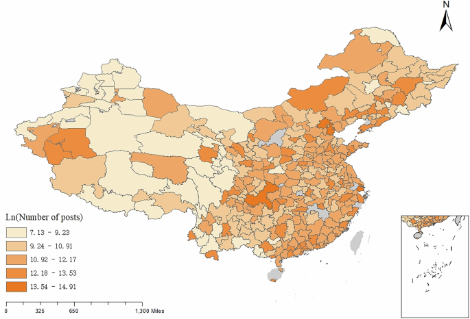
The daily PNEEC for each city was estimated using a lexicon-based semantic analysis tool applied to 45 million geocoded microblog tweets posted on SINA Weibo, the largest microblog platform in China. The extensive data set spans 335 Chinese cities from January 1, 2020, to March 31, 2020 (Fig. 1). Keywords that gained collective attention since the initial reported cases of COVID-19 were used to extract the posts containing COVID-19-related terms (see Supplementary Note 1 for details). Subsequently, we constructed the public emotional expressions related to COVID-19 for each city and day using location-based social media (LBSM) data. Since LBSM content is typically short in length and sentiment is relatively explicit and compact, noise can be filtered out more effectively, making lexicon-based sentiment analysis a more straightforward and robust approach. Specifically, for each Weibo post, we first remove all non-Chinese characters (e.g., numbers, English text, punctuation, URLs, hashtags, and mentions) and then perform Chinese word segmentation. Each segmented token is matched against a lexicon to identify its polarity (negative or positive).

The map visualizes the spatial density of COVID-19-related Weibo posts across 335 Chinese cities using log-transformed counts. Regions are shaded according to post density, with warmer colors indicating higher volume. Grey areas represent regions with missing or insufficient geocoded Weibo data.
In our main analysis, we adopt a dictionary-based algorithm utilizing the Chinese Emotional Vocabulary Ontology (CEVO), which is organized and labeled by the Information Retrieval Research Office of Dalian University of Technology. CEVO classifies each Chinese word or phrase by word type, emotion type, emotion intensity, and polarity. Its emotion classification system is grounded in Ekman’s framework, covering seven parts of speech (Noun, Verb, Adjective, Adverb, NW, Idiom, and Prepositional Phrase). Each entry is assigned one of three polarities, neutral (5,376 words), positive (11,230 words), or negative (10,784 words). Using CEVO, we extract positive and negative sentiment by counting positive and negative words. We then aggregate these values across all Weibo posts from each city on each day to calculate the total PNEEC. This approach offers a direct measure of daily sentiment at the city level.
Moreover, to verify the robustness of our results, we construct a secondary version of PNEEC using another widely employed Chinese lexicon, Hownet (published by China National Knowledge Infrastructure, CNKI). Similar to CEVO, Hownet provides polarity and intensity annotations but also allows consideration of context-specific orientations through syntactic patterns. This corpus-based enhancement helps identify whether certain terms shift their sentiment orientation in specific contexts or not. Our findings remain consistent when using Hownet for sentiment scoring, indicating that the main patterns hold regardless of the particular lexicon used (see Supplementary Note 4 for details).
Geographic, mobility and social media ties
Since public emotional expression does not occur in isolation but rather interacts through social interactions, we constructed three types of inter-city ties (geographic, mobility, and social media) to examine how emotions propagate across different relational structures.
To capture geographical ties, we constructed a binary matrix, defining two cities as geographically connected if they share a border. For mobility ties, mobility data was sourced from Tencent Location Big Data, incorporating 57 billion trips amongst 335 cities from 2015 to 2017. For social media ties, we constructed a directed inter-city attention network using 296 million real-time posts from multiple social media platforms. The data was obtained from Intelligent Starshine, a cognitive intelligence and text big data service provider, which covers major social media platforms such as Weibo, Tencent, and Tiktok. To characterize dynamic social media ties, 91 daily directed asymmetric matrices were constructed.
Pandemic phases
Understanding the dynamics of emotional interactions requires situating it within the broader timeline of the pandemic. The impact of geographic, mobility, and social media ties on public emotion likely varied across different stages of the crisis. Therefore, we categorized the pandemic into different phases to better analyze shifts in emotional expression and inter-city interactions. Based on Covid-19-related events in the United States and past research findings, Ashokkumar and Pennebaker (2021) divided this public health event into four phases: baseline phase, warning phase, isolation phase, and normalization phase. Drawing on this division criterion, on the basis of major COVID-19-related events that occurred in China (Lu et al. 2024), this study also stages the development of the pandemic in the Chinese context (see Table 1).
The warning phase spanned from January 1, 2020 to January 20, 2020. On December 31, 2019, COVID-19 was initially reported to the WHO. As more evidence emerged, official warnings were progressively updated, transitioning from simply acknowledging the possibility of human-to-human transmission to ultimately confirming it.
The isolation phase spanned from January 21, 2020 to February 29, 2020. On January 21, 2020, China’s provincial governments announced the launch of a level I (or level II) emergency response to major public health emergencies. Across China, the majority of the population self-isolated, causing daily mobility across the country to decrease by more than 70% [This is calculated based on the population migration data disclosed by Baidu: https://qianxi.baidu.com/#/2020chunyun].
The normalization phase spanned from March 1, 2020 to March 31, 2020. Past studies suggest that following an unexpected crisis, the initial surge in interest subsides about 6 weeks after the event (Ashokkumar and Pennebaker 2021). After March 1, the pandemic was essentially contained nationwide, with the number of new confirmed cases reaching zero for the first time. We observed four weeks of data (3.1–3.31) to measure the public’s risk perception in the normalization phase.
Control variables
Given the complexity of emotional interactions across cities, it is essential to control for potential confounding factors that may influence public emotions. Various epidemiological, environmental, economic, and demographic factors can shape emotional expressions, independently of social ties. To ensure the robustness of our findings and isolate the effects of geographic, mobility, and social media ties on PNEEC, we incorporated a range of control variables into our models. In this study, we implemented rigorous control measures to account for various epidemiological conditions, including cumulative confirmed cases, cumulative death cases, and cumulative cured cases. Additionally, we incorporated local policies into our models, such as travel bans, emergency declaration levels, home isolation measures, and the intensity of restrictions. Furthermore, we accounted for weather conditions, including indicators of PM2.5, temperature, and total amount of rainfall, as well as local per capita GDP, disaster experience, hospital bed capacity, aging population, internet access rate, medical insurance coverage, and the proportion of the tertiary industry. Table 2 provides the explanation of the variables studied in this study.
Methods
Moran’s I
Global Moran’s I (GI) is a statistical measure used to quantify spatial autocorrelation, originally developed by Patrick Alfred Pierce Moran. In this study, we use GI to quantify the overall spatial correlation of emotional expression among cities. Through this index, we examine whether public sentiment across different Chinese cities exhibits spatial autocorrelation based on geographic, mobility and social media ties. Furthermore, by tracking the temporal changes of GI, we reveal how emotional interactions evolved across different stages of the pandemic.
We adopt a two-stage regression framework to examine the spatial correlation of PNEEC across cities. In the first stage, we regress PNEEC data (from Day 1 to Day 91) on the time trend term and all relevant local pandemic variables, thereby obtaining the residuals (Residualit) from the first-stage regression. These residuals represent the deviation between observed and predicted values, capturing the variance unexplained by local pandemic-related factors. In other words, they represent the component of PNEEC not attributable to pandemic-related factors. In the second stage, these residuals are used to calculate GI. By focusing on the residuals, we effectively filter out the emotional correlation directly driven by the pandemic’s spatial association.
Where ({varphi }_{t}) denotes the time trend item; ({{Residual}}_{{it}}) is the value of ({Residual}) in city (i) at date (t); ({overline{{Residual}}}_{t}) is the average value of ({Residual}) with the sample number of 335 at date (t); ({{Residual}}_{{jt}}) is the value of the variable ({Residual}) at all the other locations (where (jne i)) at date (t); ({omega }_{{ijt}}) denotes the spatial weight, defined by the existence of geographic, mobility, or social media ties between cities (i) and (j) on date (t) (see details in Supplementary Note 1), and ({S}_{t}^{0}) is the sum of all ({omega }_{{ijt}}) at date (t).
Negative/positive values of GI indicate negative/positive spatial autocorrelation. Values range from −1 (indicating perfect dispersion) to 1 (perfect correlation). A zero value indicates a random spatial pattern. A GI value close to +1 indicates strong positive spatial autocorrelation. This means values cluster together. For example, elevation datasets have similar elevation values close to each other. Negative spatial autocorrelation occurs when GI is near −1. A checkerboard is an example where Moran’s I is −1 because dissimilar values are next to each other. A value of 0 for GI typically indicates no autocorrelation.
Local Moran’s enables identification of localized emotional correlation between a given city (i) and its neighboring cities.
A high positive value of Local Moran’s I suggests that the PNEEC of city (i) is similar in magnitude (either high or low) to that of its neighboring cities, thus the cities are spatial clusters. Spatial clusters include high–high clusters and low–low clusters. A high negative LI value means that the PNEEC of city i is a spatial outlier. Spatial outliers are those values that are obviously different from the values of their surrounding cities, which means low emotional interaction.
Regression discontinuity design
Regression discontinuity (RD) is a useful method for identifying the causal impact of a treatment assigned according to a known rule that consists of a cutoff in an assignation or forcing variable. It makes use of the assumption that units which just qualify for treatment are similar to those which just miss out on treatment, such that average differences in the outcomes of those individuals sufficiently close to either side of the cutoff point can be attributed to the treatment.
Two cutoff dates, January 20th of and February 28th, mark the transitions into the isolation and normalization stages of the COVID-19 pandemic. We adopt a parametric approach to estimate the treatment effect (Jacob et al. 2012), using all relevant observations to model the outcome variable LIit (i.e., the Local Moran’s I for city (i) on day (t)), as a function of the forcing variable, the number of days from the cutoff date. The baseline regression discontinuity design is specified as follows:
In model (3), ({{LI}}_{{it}}) denotes the Local Moran’s I of public negative emotional expressions about COVID-19 for city i on day t. The treatment variable ({T}_{{it}}) equals 1 if the observation belongs to the treatment group, and 0 otherwise. The forcing variable ({X}_{{it}}) represents the number of days from the cutoff date for city i. The polynomial term ({({X}_{{it}})}^{p}), along with their corresponding coefficients ({gamma }_{p}) (control) and ({gamma }_{p}^{{prime} }) (treatment), capture potential nonlinear trends and allow for different functional forms on either side of the cutoff. ({varepsilon }_{{it}}) is the random error term.
In model (4), ({T}_{{it}}^{{prime} }) is the treatment variable, representing the mitigation of the pandemic.
In the parametric regression discontinuity design (RDD) approach, there is no consensus regarding the appropriate polynomial order. Since there is no specific reason to assume a linear functional form, researchers often employ higher-order polynomial regression models in practice (Gelman and Imbens 2019). For example, Black et al. (2007) used fourth-order polynomials to evaluate the U.S. Worker Profiling and Reemployment Services system. Chen et al. (2013) applied a parametric approach to examine the impact of coal-induced air pollution during winter on residents’ life expectancy north of Huaihe River, increasing the polynomial order up to five. According to the research of Gelman and Imbens (2019), among 29 empirical studies using parametric RDD approach in top-tier economics journals, the polynomial order was generally set to five or below. Accordingly, this study sets the maximum polynomial order to five and reports results for polynomial orders one through five. Given the sensitivity of parametric results to polynomial order, we selected the model with the smallest AIC value as the optimal specification, following Bronzini and Iachini (2014). The estimated coefficient (beta) for the treatment indicators ({T}_{{it}}) and ({T}_{{it}}^{{prime} }) are the primary parameters of interest in this study, capturing the changes in cities’ emotional connectivity at key discontinuity points associated with the pandemic’s progression.
Spatial autocorrelation and interaction models
Referring to Konisky (2007), we estimate a series of interaction models to test whether a city’s PNEEC is a function of that of its network neighbor. First, we construct a baseline spatial autoregressive model as follows:
Where the dependent variable, ({{rm{PNEEC}}}_{{it}}), denotes the negatively expressed public emotion about COVID -19 in city (i) at date (t) and ({{rm{PNEEC}}}_{{jt}}) is negative public expressed emotion of COVID -19 in city (j) at date (t), not including city (i) itself. ({omega }_{{ijt}}) denotes the weight assigned to city (j) by city (i) at time (t), based on the geographic, mobility, or social media matrix (see details in Supplementary Note 1). ({X}_{{it}}) is the vector of host city characteristics including epidemiological variables, policy variables, and weather variables. ({phi }_{i}) represents city fixed effects, and ({varphi }_{t}) represents date fixed effects, ({varepsilon }_{{it}}) are independently normally distributed error terms with ({rm{E}}left[{varepsilon }_{{it}}right]=0) and (mathrm{var}left[{varepsilon }_{{it}}right]={sigma }^{2}). Equation (5) serves as the baseline model for testing the spatial autocorrelation of PNEEC, with the spatial lag term (sum {omega }_{{ijt}}{{rm{PNEEC}}}_{{jt}}) as the primary variable of interest.
Further, we study the interaction pattern of PNEEC reflected of city responsiveness. We estimate an additional model to test the interaction effects in city-level responsiveness. Equation (6) tests whether PNEEC interactions among cities intensifies when the average PNEEC in neighboring cities declines compared to the previous day. We develop a two-stage regression framework to examine the interaction effect.
where
The definitions of the variables remain consistent with those in Eq. (5). According to Eq. (6), when the weighted average of neighboring cities’ PNEEC is lower than that of the previous day, ({D}_{{it}}) = 1, and the coefficient ({delta }_{0}) captures the interaction effect when emotional responses intensify under declining neighbor sentiment. If the weighted average of neighboring cities’ PNEEC increases relative to the previous day, ({D}_{{it}}) = 0, otherwise, the interaction effect is captured by ({delta }_{1}).
PVAR and forecast error variance decomposition
To assess the differential contributions of geographic, mobility, and social media neighbors’ PNEEC to local PNEEC, we employed a Panel Vector Autoregression (PVAR) model and used Forecast Error Variance Decomposition (FEVD) to examine the contribution of each variable.
A PVAR model was estimated as follows. The endogenous variables include PNEEC from geographic (({{rm{PNEEC}}}_{{it}}^{{geo}})), mobility (({{rm{PNEEC}}}_{{it}}^{{mob}})), and social media neighbors (({{rm{PNEEC}}}_{{it}}^{{soc}})), as well as the local city’s own PNEEC (({{rm{PNEEC}}}_{{it}})). The PVAR model is:
where
In Eq.(7), t denotes the date ((t=mathrm{1,2},cdots ,91)), and (i) denotes the local city; ({beta }_{m,n}^{{ij}}) ((m,n=mathrm{1,2,3,4})) are coefficients; ({alpha }_{m}^{i}) are constants that represent panel fixed-effects; ({varepsilon }_{{mt}}^{i}) are idiosyncratic errors; k is an optimal lag length of the model; ({{rm{PNEEC}}}_{{jt}}) is negative public expressed emotion of COVID -19 in city j at date t, not including city (i) itself. ({omega }_{{ij}}^{{geo}}), ({omega }_{{ij}}^{{mob}}), and ({omega }_{{ijt}}^{{soc}}) denote the weight assigned to city (j) by city (i) at time (t) using the geographic, mobility, and social media matrix (see details in Supplementary Note 1). The optimal lag length (k) was determined to be 1 based on the smallest values of the Akaike information criteria (AIC) and the Bayesian information criteria (BIC). In order to remove panel-specific fixed effects, we applied forward orthogonal deviation or Helmert transformation on these variables. This method transforms variables by means of forward mean-differencing and ensures orthogonality between transformed variables and lagged variables. In the PVAR model, coefficients indicate the relationship between lagged variables and the variables on the left side of the equation. We emplyed GMM-style instruments to improve the estimation accuracy of the model (Holtz-Eakin et al. 1988).
FEVD examines the contribution of each variable on the right side of the above equation to the ones on the left side. FEVD provides variance contribution metrics analogous to R2 statistic, reflecting the explanatory power of each endogenous variable. We applied FEVD to the PVAR model. FEVD results reveal that neighbors’ PNEEC influenced local PNEEC to varying degrees across different relational dimensions.
Results
The effect of the pandemic on PNEEC and GI of PNEEC
Cointegration tests reveal full or partial cointegration relationships among the PNEEC of 335 cities. We then computed the GI of PNEEC across geographic, mobility, and social media ties (Fig. 2). Notably, PNEEC exhibits significant spatial autocorrelation across all three ties. The GI of PNEEC exhibits phase-specific fluctualtions that appear to correspond with the number of reported COVID-19 cases (the shaded area in Fig. 2). This observation aligns with Stevenson and Taylor (2018)’s suggestion to consider the multistage process in risk communication, with crises progressing through distinct stages (Xu et al. 2020). The pandemic was categorized into three stages based on Ashokkumar and Pennebaker (2021)’s division criteria: the warning phase, isolation phase, and normalization phase, with distinct GI patterns observed across these stages.

This figure shows the daily changes in global Moran’s I of public negative emotional expression about the pandemic (PNEEC) from January 1 to March 31, 2020, across three types of social ties. The grey shaded area denotes newly confirmed domestic COVID-19 cases (excluding imported cases). Time trends and pandemic-related covariates are controlled for in the model.
Under both geographic and mobility ties, the GI indicates positive spatial interaction of PNEEC. During the warning stage, GI values are more volatile (SD = 0.079 for geographic ties and 0.055 for mobility ties) compared to the isolation stage (SD = 0.050 for geographic and 0.044 for mobility ties). Moreover, the average GI during the isolation stage (0.245 for geographic and 0.186 for mobility ties) is notably lower than during the normalization stage (0.559 for geographic and 0.374 for mobility ties), suggesting that spatial interaction of PNEEC was both weaker and more stable during the isolation stage.
In the social media tie, GI fluctuates sharply during the warning stage, while it is close to 0 and not significant during the isolation stage. This indicates that during the isolation stage, the PNEEC in neighboring areas is not related to the local PNEEC in the social media tie. However, during the normalization stage, a significantly negative interaction is observed, with a mean value of −0.161, implying negative spatial correlation of PNEEC.
Table 3 presents the regression results of Models (4) and (5) across Panels A, B, and C, corresponding to geographic, mobility and social media ties, respectively, with LI as the dependent variable. The estimated coefficient of treatment variable-isolation is consistently significant across different polynomial orders and sample ranges. However, the estimated coefficient of treatment variable-normalization is not significant. Based on AIC tests, relatively low polynomial order (e.g., 2 or 1) is supported. Panel B reveals the causal impact of the pandemic’s isolation and normalization on PNEEC correlations in geographic ties, with a first-order polynomial model being the optimal fit. The estimated coefficients of treatment variables (isolation and normalization of the pandemic) are significant at the 95% confidence level. The results, combined with Fig. 3, indicate that both the isolation and normalization stages significantly increase PNEEC interactions in geographical ties. This suggests a high level of communal relationship attributes among geographically adjacent cities, motivating joint efforts to control and prevent the pandemic.

The panels show regression discontinuity plots capturing shifts in spatial emotional correlation before and after key pandemic milestones (outbreak and mitigation). Each plot is constructed using either 60 bins (panel a) or 70 bins (panel b), and estimated using a local polynomial regression with a triangular kernel. Pointwise 95% confidence intervals are displayed.
Panel C illustrates the effects of the pandemic’s isolation and normalization stages on PNEEC interactions through mobility ties. The outbreak of the pandemic had no significant impact on PNEEC interaction, whereas normalization significantly increased positive interactions. After initial pandemic control, people may share a common motivation with their mobility neighbors to return to normal life and work, fostering increased positive interactions in PNEEC.
Panel D reveals that the impacts of pandemic isolation and normalization on PNEEC interactions in social media ties are not significant. However, as shown in Fig. 3a, PNEEC interaction within social media ties significantly decreased five days prior to the pandemic outbreak, possibly due to the official Health Commission’s initial release of information on limited human-to-human transmission. This indicates that individuals in social media ties display heightened sensitivity compared to those in geographic and mobility ties. Although the results were not statistically significant, a trend suggests that pandemic mitigation was associated with increased negative PNEEC interaction (Fig. 3b). This observation implies a lack of common motivation among individuals in social media ties, leading to negative comparisons. The assessment of the internal validity of the RD design can be seen in Supplementary Note 2.
Overall, our findings shed light on the effect of the pandemic on PNEEC and its spatial autocorrelation across different ties. The results provide valuable insights into emotional interactions among cities during the pandemic, contributing to a deeper understanding of public emotional responses and behaviors in risky situations.
The interactions of PNEEC among cities in three social ties
In this section, we delve deeper into the interactions of PNEEC among cities in geographic, mobility, and social media ties. Figure 4 represents the results of Eq. (6), formulated in the ‘Interaction model’ section of the Methods. The coefficients δ0 and δ1 represent the local PNEEC feedback coefficients when the PNEEC of neighbors increases or decreases by 1%, respectively. Our analysis reveals distinct patterns of PNEEC feedback in different social ties.

The bar plots display standardized spatial interaction coefficients of PNEEC under warning, isolation, and normalization stages across three social tie types. The coefficients are estimated using OLS regressions based on Eq. (6), controlling for city/date fixed effects and pandemic, policy, and weather covariates. The results are derived from 18 separate regressions across different subsamples and interaction terms.
First, we observe amplified positive feedback in social media ties during the warning stage. Specifically, when the PNEEC of neighbors increases by 1%, the local PNEEC rises by 1.128% ((left.{rm{delta }}0=1.128;{{P}} < 0.001right)).
Second, in geographic ties, we find shrinking positive feedback of local PNEEC. When the PNEEC of neighbors rises or falls by 1%, the local PNEEC positively responds by less than 1%. For instance, during the isolation stage, the local PNEEC feedback coefficients are both below 0.5 (δ0 = 0.451, P < 0.001; δ1 = 0.345, P <0>
Third, negative feedback is evident in social media ties during the normalization stage. When the PNEEC of neighbors increases by 1%, the local PNEEC decreases by 0.162% (δ1 = 0.162, P < 0.001).
Finally, we observe asymmetry in the mobility ties, where local PNEEC responds differently to increases and decreases in neighbors’ PNEEC. The local response to rising PNEEC in neighbors is much stronger than its response to a decline. For instance, at the normalization stage, the local response coefficients to increases and decreases in neighbors’ PNEEC are 0.401 and 0.316, respectively (see Fig. 4).
To further explore the dynamics of PNEEC interactions across different types of social ties in various pandemic stages, we constructed a PVAR model with four endogenous variables related to PNEEC (local, geographic neighbors, mobility neighbors, social media neighbors). Through the method of FEVD, we examined the relative contribution rate of neighbors’ PNEEC to variations in local PNEEC. The FEVD results highlight how PNEEC interactions depend on different types of ties across pandemic stages.
As illustrated in Fig. 5, social media neighbors exert the most significant contribution to local PNEEC changes during the warning stage, exceeding the combined influence of mobility and geographic ties. Subsequently, the contribution rate of social media neighbors gradually decreases, reaching below 10% in the normalization stage. In contrast, the contribution rate of geographical neighbors shows a trend of gradual increase. Notably, after the outbreak of the pandemic on January 20, the contribution rate of geographic neighbors rapidly rises from 40% to over 60%. In the normalization stage, the contribution rate of geographic neighbors remains at a high level of more than 45%. The contribution rate of mobility neighbors remains relatively stable in the first two stages. Combining this with the absolute contribution value (see Supplementary Note 3), we observe that the total contribution rate during the isolation stage is lower than that during the warning and normalization stages.

This figure presents the forecast error variance decomposition (FEVD) results from the PVAR model, showing how geographic, mobility, and social media neighbors contributed to local PNEEC over time. The horizontal axis indicates time (days), and the vertical axis represents the relative contribution of each tie type. The decomposition is shown separately for the warning, isolation, and normalization phases.
These findings provide valuable insights into the dynamics of PNEEC interactions among cities in different social ties during distinct stages of the pandemic, contributing to a better understanding of the influence of social networks on emotional responses in times of crisis.
Discussion and conclusion
The COVID-19 pandemic has presented a unique opportunity to study the emotional relationships among cities on a massive scale. The coordination and cooperation required during this period have reshaped the nature of geographic, mobility, and social media ties. When communities or cities collaborate to contain the virus, they develop a sense of communal relationship attributions within these ties. This shared sense of responsibility leads to more pronounced emotional interactions in geographic ties than those in mobility or social media ties. The significance of this finding lies in acknowledging the pivotal role of communal relationships in shaping emotional dynamics during crises,. This finding align with previous research by Clark and Mills (2011), which emphasizes the importance of communal relationships in social interactions.
This research contributes to the literature in three major ways. First, it expands our understanding of intercity emotional interactions during a global crisis in the context of COVID-19. By examining large-scale data from geographic, mobility, and social media ties, this study reveals the complex emotional dynamics that emerge among cities facing a common public health threat. These insights demonstrate how different types of ties influence emotional responses during a crisis, offering practical implications for both crisis management and coordination.
Second, we identify the impact of social ties on emotional interactions. By investigating three types of ties (geographic, mobility, and social media) the study uncovers distinct levels of emotional interplay among cities. The finding that geographic ties exhibit higher emotional interactions than mobility or social media ties highlights the significance of physical proximity and shared responsibilities in shaping emotional responses.
Third, these findings offer practical implications for improving crisis management and coordination. The study underscores the importance of cross-regional emergency collaboration during large-scale disasters. Understanding how emotional interactions occur between cities can inform strategies for crisis management, enabling more coordinated and effective responses to comparable public health emergencies or other widespread disasters. By recognizing how communal relationship factors influence emotional connections, authorities can strengthen a collective sense of responsibility and foster cooperation across cities, thereby enhancing both crisis response and prevention measures.
The study contributes to the literature on emotions, social ties, and crisis management by providing empirical evidence of intercity emotional interactions during the COVID-19 pandemic. In particular, it uniquely integrates social media data with mobility patterns to offer a more holistic view of public emotional dynamics, demonstrating how digital platforms and mobility flows interact to shape collective responses. The findings highlight the need to consider communal relationships and shared responsibilities when examining emotional responses to public health crises. This perspective offers practical implications for policymakers and crisis-response authorities. By leveraging social media insights and understanding the dynamics of emotional interactions, officials can better anticipate and address societal concerns, misconceptions, and emotional reactions, ultimately improving compliance with health guidelines and bolstering crisis management. Furthermore, this research emphasizes the significance of cross-regional emergency coordination and calls attention to potential emotional interactions and polarization during large-scale, rapidly spreading disasters. Overall, it enriches our understanding of emotional responses and behaviors under high-risk conditions, providing valuable guidance for enhancing crisis management mechanisms in future emergencies.
In summary, our evidence supports the conclusion that the urban population’s PNEEC is correlated among cities during the COVID-19 pandemic and is influenced by intercity ties. The availability of social media has facilitated the expression of emotions following a public crisis, and government agencies have utilized these platforms to guide public behavior through emotional regulation. Crucially, our study focuses on emotions closely tied to COVID-19, which affect individuals’ views of the virus and their adoption of self-protective measures. Furthermore, the interactions of social media-based emotional expressions between cities underscore the importance of cross-regional emergency coordination. In large-scale disasters such as infectious disease outbreaks, river basin floods, or wildfires, it is vital to consider emotional interactions among different regions. The coordination demanded by disaster prevention and control efforts can transform the foundational attributes of ties among regions, potentially prompting emotional interactions and polarization.While our study offers valuable insights into the emotional interaction patterns observed during the pandemic, several limitations must be acknowledged. First, although the linguistic measure derived from natural language processing (NLP) is useful as a proxy for emotions, it may still introduce noise. We addressed this concern through robustness checks using different NLP methods (see Supplementary Note 5), yet the possibility of errors remains. Second, our use of specific keywords on Weibo to filter COVID-19-related posts may have excluded some relevant emotional expressions, potentially underestimating certain aspects of pandemic-related sentiment. Third, social media users are not fully representative of the broader population, as they tend to be younger and more educated. This demographic skew may overstate the prevalence or intensity of emotional interactions in various ties. Although we accounted for demographic effects such as aging in our analyses, a comprehensive picture of emotional expressions may require additional data sources. Finally, the study primarily focuses on COVID-19-specific emotions, which directly shape individuals’ perceptions and behaviors related to the coronavirus, but may not fully capture broader emotional or psychological responses to crises in general.
Given these limitations, future research could take several directions. First, more comprehensive sentiment analysis approaches or datasets could be employed to capture a broader range of emotional expressions and reduce potential measurement bias. Expanding to additional social media platforms or integrating offline data (e.g., surveys, interviews, or ethnographic methods) could help verify and generalize the findings beyond the Weibo user demographic. This step would also illuminate how observed digital patterns replicate in the physical world, where matching specific interactions can be complex. Second, exploring the role of social bubbles could offer deeper insight into how small, tightly knit communities influence emotional contagion under rapidly changing conditions, such as lockdowns or partial reopenings. Evidence from Buchel et al. (2021) and Leng et al. (2021) suggests that social bubbles can serve as psychological buffers, shaping the intensity and direction of emotional interactions. Future studies could examine whether and how these bubble-based interactions affect intercity emotional convergence or divergence during different stages of a crisis. Third, longer or multiple time windows could be investigated to determine how emotional interactions evolve under various phases of a crisis or in comparison to non-crisis periods. Fourth, cross-cultural or cross-national analyses would shed light on whether communal relationship dynamics, social bubbles, and emotional contagion patterns vary across cultural contexts or governance structures. Finally, investigating real-time feedback loops, where emotional expressions affect policies and, in turn, reshape emotional contagion, could yield practical insights for adaptive crisis management strategies.
In conclusion, our research sheds light on the dynamics of emotional interactions among cities during the pandemic and highlights the role of social ties in shaping these interactions. Understanding these emotional dynamics can inform crisis management strategies and enhance cross-regional emergency coordination in the face of similar large-scale disasters.
Data availability
The datasets and code generated and analyzed during the current study are available from the corresponding author upon reasonable request.
References
-
Ashokkumar A, Pennebaker JW (2021) Social media conversations reveal large psychological shifts caused by COVID-19’s onset across US cities. Sci Adv 7(39):eabg7843
-
Baek EC, Parkinson C (2022) Shared understanding and social connection: Integrating approaches from social psychology, social network analysis, and neuroscience. Soc Personal Psychol Compass 16(11):e12710
-
Bavel JJV, Baicker K, Boggio PS, Capraro V, Cichocka A, Cikara M, Druckman JN (2020) Using social and behavioural science to support COVID-19 pandemic response. Nat Hum Behav 4(5):460–471
-
Black DA, Galdo J, Smith JA (2007) Evaluating the worker profiling and reemployment services system using a regression discontinuity approach. Am Economic Rev 97(2):104–107
-
Bond RM, Bushman BJ (2017) The contagious spread of violence among US adolescents through social networks. Am J Public Health 107(2):288–294
-
Bronzini R, Iachini E (2014) Are incentives for R&D effective? Evidence from a regression discontinuity approach. Am Economic J: Economic Policy 6(4):100–134
-
Buchel O, Ninkov A, Cathel D, Bar-Yam Y, Hedayatifar L (2021) Strategizing COVID-19 lockdowns using mobility patterns. R Soc Open Sci 8(12):210865
-
Catania G, Zanini M, Hayter M, Timmins F, Dasso N, Ottonello G, Bagnasco A (2021) Lessons from Italian front‐line nurses’ experiences during the COVID‐19 pandemic: A qualitative descriptive study. J Nurs Manag 29(3):404–411
-
Chen Y, Ebenstein A, Greenstone M, Li H (2013) Evidence on the impact of sustained exposure to air pollution on life expectancy from China’s Huai River policy. Proc Natl Acad Sci 110(32):12936–12941
-
Clark MS, Mills JR (2011) A theory of communal (and exchange) relationships. Handb theories Soc Psychol 2:232–250
-
Fowler JH, Christakis NA (2008) Dynamic spread of happiness in a large social network: longitudinal analysis over 20 years in the Framingham Heart Study. BMJ 337:a2338
-
Garcia D, Rimé B (2019) Collective emotions and social resilience in the digital traces after a terrorist attack. Psychological Sci 30(4):617–628
-
Gelman A, Imbens G (2019) Why high-order polynomials should not be used in regression discontinuity designs. J Bus Economic Stat 37(3):447–456
-
Hale T, Angrist N, Goldszmidt R, Kira B, Petherick A, Phillips T, Majumdar S (2021) A global panel database of pandemic policies (Oxford COVID-19 Government Response Tracker). Nat Hum Behav 5(4):529–538
-
Hatfield E, Cacioppo JT, Rapson RL (1993) Emotional contagion. Curr directions psychological Sci 2(3):96–100
-
Holtz-Eakin D, Newey W, Rosen HS (1988) Estimating vector autoregressions with panel data. Econometrica: J Econometric Soc 56(6):1371–1395
-
Jacob R, Zhu P, Somers M-A, Bloom H (2012) A practical guide to regression discontinuity. MDRC
-
Kahneman D, Krueger AB (2006) Developments in the measurement of subjective well-being. J Economic Perspect 20(1):3–24
-
Konisky DM (2007) Regulatory competition and environmental enforcement: Is there a race to the bottom? Am J Political Sci 51(4):853–872
-
Kramer AD, Guillory JE, Hancock JT (2014) Experimental evidence of massive-scale emotional contagion through social networks. Proc Natl Acad Sci 111(24):8788–8790
-
Le BM, Impett EA, Lemay Jr EP, Muise A, Tskhay KO (2018) Communal motivation and well-being in interpersonal relationships: An integrative review and meta-analysis. Psychological Bull 144(1):1
-
LeDoux J (2012) Rethinking the emotional brain. Neuron 73(4):653–676
-
Leng T, White C, Hilton J, Kucharski A, Pellis L, Stage H, Flasche S (2021) The effectiveness of social bubbles as part of a Covid-19 lockdown exit strategy, a modelling study. Wellcome open Res 5:213
-
Logemann M, Aritz J, Cardon P, Swartz S, Elhaddaoui T, Getchell K, Palmer‐Silveira JC (2022) Standing strong amid a pandemic: How a global online team project stands up to the public health crisis. Br J Educ Technol 53(3):577–592
-
Lu L, Xu J, Wei J, Shults FL, Feng XL (2024) The role of emotion and social connection during the COVID-19 pandemic phase transitions: a cross-cultural comparison of China and the United States. Humanities Soc Sci Commun 11(1):1–16
-
Ogunfowora B, Weinhardt JM, Hwang CC (2021) Abusive supervision differentiation and employee outcomes: The roles of envy, resentment, and insecure group attachment. J Manag Inf Syst 47(3):623–653
-
Peeri NC, Shrestha N, Rahman MS, Zaki R, Tan Z, Bibi S, Haque U (2020) The SARS, MERS and novel coronavirus (COVID-19) epidemics, the newest and biggest global health threats: what lessons have we learned? Int J Epidemiol 49(3):717–726
-
Perlman S (2020) Another decade, another coronavirus. N. Engl J Med 382(8):760–762
-
Rimé B (2009) Emotion elicits the social sharing of emotion: Theory and empirical review. Emot Rev 1(1):60–85
-
Rosenquist JN, Fowler JH, Christakis NA (2011) Social network determinants of depression. Mol psychiatry 16(3):273–281
-
Rottenstreich Y, Hsee CK (2001) Money, kisses, and electric shocks: On the affective psychology of risk. Psychological Sci 12(3):185–190
-
Slovic P, Finucane ML, Peters E, MacGregor DG (2013) Risk as analysis and risk as feelings: Some thoughts about affect, reason, risk and rationality. In The feeling of risk (pp. 21-36): Routledge
-
Slovic P, Peters E (2006) Risk perception and affect. Curr directions psychological Sci 15(6):322–325
-
Stevenson M, Taylor B (2018) Risk communication in dementia care: family perspectives. J Risk Res 21(6):692–709
-
Thibaut JW (2017) The social psychology of groups. Routledge
-
Valdez D, Ten Thij M, Bathina K, Rutter LA, Bollen J (2020) Social media insights into US mental health during the COVID-19 pandemic: Longitudinal analysis of Twitter data. J Med Internet Res 22(12):e21418
-
Van Der Velden PG, Contino C, Das M, Leenen J, Wittmann L (2022) Differences in mental health problems, coping self-efficacy and social support between adults victimised before and adults victimised after the COVID-19 outbreak: population-based prospective study. Br J Psychiatry 220(5):265–271
-
Waters L, Algoe SB, Dutton J, Emmons R, Fredrickson BL, Heaphy E, Pury C (2022) Positive psychology in a pandemic: Buffering, bolstering, and building mental health. J Posit Psychol 17(3):303–323
-
Wellenius GA, Vispute S, Espinosa V, Fabrikant A, Tsai TC, Hennessy J, Boulanger A (2021) Impacts of social distancing policies on mobility and COVID-19 case growth in the US. Nat Commun 12(1):3118
-
Wise T, Zbozinek TD, Michelini G, Hagan CC, Mobbs D (2020) Changes in risk perception and self-reported protective behaviour during the first week of the COVID-19 pandemic in the United States. R Soc open Sci 7(9):200742
-
World Health Organization (2022) COVID-19 pandemic triggers 25% increase in prevalence of anxiety and depression worldwide. World Health Organization. https://www.who.int/news/item/02-03-2022-covid-19-pandemic-triggers-25-increase-in-prevalence-of-anxiety-and-depression-worldwide
-
Xu L, Qiu J, Gu W, Ge Y (2020) The dynamic effects of perceptions of dread risk and unknown risk on SNS sharing behavior during EID events: Do crisis stages matter. J Assoc Inf Syst 21(3):545–573
-
Zhang X, Yang Q, Albaradei S, Lyu X, Alamro H, Salhi A, Tifratene F (2021) Rise and fall of the global conversation and shifting sentiments during the COVID-19 pandemic. Humanities Soc Sci Commun 8(1):1–10
Acknowledgements
This research was funded by the National Science Foundation of China (No.72374066, 72474064, 72004213).
Author information
Authors and Affiliations
Contributions
Conceptualization, LL, JX and JW; Data curation, LL, JX and JW; Formal analysis, LL, JX and JW; Writing – original draft, LL and JX; Writing – review & editing, LL, JX and JW. All authors commented on previous versions of the manuscript. All authors read and approved the final manuscript.
Corresponding author
Ethics declarations
Competing interests
The authors declare no competing interests.
Ethical approval
This article does not contain any studies with human participants performed by any of the authors.
Informed consent
This article does not contain any studies with human participants performed by any of the authors.
Additional information
Publisher’s note Springer Nature remains neutral with regard to jurisdictional claims in published maps and institutional affiliations.
Supplementary information
Rights and permissions
Open Access This article is licensed under a Creative Commons Attribution-NonCommercial-NoDerivatives 4.0 International License, which permits any non-commercial use, sharing, distribution and reproduction in any medium or format, as long as you give appropriate credit to the original author(s) and the source, provide a link to the Creative Commons licence, and indicate if you modified the licensed material. You do not have permission under this licence to share adapted material derived from this article or parts of it. The images or other third party material in this article are included in the article’s Creative Commons licence, unless indicated otherwise in a credit line to the material. If material is not included in the article’s Creative Commons licence and your intended use is not permitted by statutory regulation or exceeds the permitted use, you will need to obtain permission directly from the copyright holder. To view a copy of this licence, visit http://creativecommons.org/licenses/by-nc-nd/4.0/.
About this article

Cite this article
Xu, J., Lu, L. & Wei, J. The impact of geographic, mobility and social media ties on massive-scale regional public emotional interaction.
Humanit Soc Sci Commun 12, 883 (2025). https://doi.org/10.1057/s41599-025-05280-2
-
Received:
-
Accepted:
-
Published:
-
DOI: https://doi.org/10.1057/s41599-025-05280-2
This post was originally published on this site be sure to check out more of their content