Unveiling the social fabric through a temporal, nation-scale social network and its characteristics

Interactions between individuals are at the core of social life. Consequently, researchers across many different fields have long been interested in understanding the structure of these interactions, i.e., social networks^1,2,3,4. This is an inherently challenging task as social interactions are rarely directly observed by researchers and are difficult to reproduce in an experimental setting. Thus, until fairly recently our understanding of social network structures was based on surveys where participants are asked to self-report with whom they interact^5,6,7. This type of data collection is, however, limited in scope and prone to multiple types of bias.

Within the last two decades, the advent of digital media and mobile phones has led to the possibility of deriving graphs from digital trace interaction data, allowing researchers to examine these structures at scale and without inherent self-reporting bias^{5,8,9,10,11,12}. However, these social networks derived from media platforms often suffer from algorithmic distortions, platform-specific behavior, and self-selected, non-random populations. These factors limit the generalizability of findings to a better understanding of broader social structures¹³.

At the same time, continuous improvements in the granularity and scope of administrative data collection have made it possible to establish network structures based on real-life social foci, i.e., entities around which joint activities are organized¹⁴. Harvey et al.¹⁵ utilize census data from New Zealand and probabilistically infer dwelling, school and work layers into a multiplex network to model COVID-19 contagion. Moving from probabilistic construction to full individual-level information, van der Laan et al.¹⁶ recently created a network of the entire population in the Netherlands by linking individuals through common households, neighborhoods, companies, educational institutions, and family relationships. While these types of networks do not capture realized social interactions, they depict the current opportunity structures for forming relationships on a national scale. This means that two individuals that are connected via any (or multiple) of those layers, have a much higher likelihood of being connected to each other in real life as opposed to any random pair in the data. The use of registry data presents immense possibilities as next to its massive scale, unselected nature and the inclusion of several social foci, registry data allows the addition of a wide variety of individual-level socio-economic and health-related information to the network. Consequently, these network data can aid the study of large-scale social phenomena and epidemiological questions. Importantly, individuals change their social foci throughout their lifetime, e.g., they change workplace or home address. As a result, network structures are highly dynamic and path-dependent. Considering that connections formed in the past, such as former classmates and colleagues, continue to hold relevant social information, it is important to incorporate a temporal dimension when studying social networks. One limitation of existing approaches leveraging administrative data for this purpose is their focus on a single point in time¹⁶.

A further challenge is the increasing amount of computational resources needed to analyze networks based on vast amounts of data, especially when relying on representations where edges indicate connections between individuals only^9,16. Here, we see a massive opportunity for improvement by leveraging the bipartite nature of administrative network data for representing social networks¹⁷.

In this paper, we present a nation-scale network for the entire population of Denmark derived from registry data for every year between 2008 and 2021. To address the first challenge of the missing temporal dimension, we introduce the concept of time-span, i.e., including edges from multiple years of administrative social networks. We use this framework to investigate how the network’s structure changes over different time horizons, conceptually akin to assuming different durability scopes of individual relationships. We address the second challenge of computational intractability by developing a novel representation of administrative networks that reflects the inherent structure of the network. Relationships in administrative networks are formed over shared foci, such as common workplaces, school classes, or nearby addresses¹⁴. In this picture, edges can also be viewed as individual’s relations to these foci, e.g., working for a specific employer in the workplace layer. We discuss how this bipartite view on administrative networks leads to a massive reduction of edges and, thus, to an increase in performance for many commonly used network algorithms. A further challenge in using administrative networks is that it is not clear to what extent people communicate in different layers, e.g., with people in their neighborhoods compare to say colleagues or classmates. Our computational framework allows for weighting edges to more plausibly reflect distances between individuals in these networks.

In our analysis, we show that the temporal stability of edges varies substantially depending on the nature of the relation. As a consequence, the level to which nodes accrue edges over time also differs, leading to increasing layer-level degree inequality. The addition of the temporal dimension also leads to reduced average shortest-paths when considering individual layers. Using the weighting scheme to adjust for the unrealistic inflation of edges, combining the different layers into one large network yields a shortest-path distribution similar to other realized social networks. Next, we point to the fact that most layers are also spatially dependent and demonstrate a strong relation between spatial proximity and edge-probability within our network. Furthermore, we show that the extent to which the degree reflects income levels for different age cohorts increases with the introduction of time-span. This finding illustrates how the properties of the network and the added time dimension encode actual life outcomes of individuals.

The aim of this study is to present this novel dataset to the research public, explore its key properties, and add to the conceptual understanding of administrative networks via a dual view, which reduces the computational burden of working with these networks. Our work should encourage further research with this network and this is why all researchers can request access to the network as well as the software to create and utilize the novel representation, via Statistics Denmark (see how to access the data in section “Data access” and the use of the software in section “Software and Python package”)¹⁸.

This section delineates the construction of a temporal, nation-scale network based on registry data, outlining the multi-dimensional structuring of nodes and edges to create diverse subnetworks for dynamic and layered analysis. Network science defines networks in terms of graphs, consisting of entities referred to as nodes and links between them, referred to as edges. In social networks, nodes frequently represent individuals and the edges describe some type of social interaction, e.g., a friendship on a social media platform. The network we construct is not based on a single definition for all nodes and edges but differentiates along multiple dimensions—two different views, time and the relation type also referred to as layer. We will introduce each of these dimensions in the following.

A dual view on the same information: individual-centered and bipartite

We introduce several fundamental, commonly shared foci as layers in a nation-scale network based on registry-data, in particular families, educational settings, workplaces, neighborhoods, and households¹⁴. We adopt a dual view on the individuals and their shared foci settings. In the first (unipartite or individual-centered view), we focus on individuals and abstract away the foci via which they can form interactions. In this perspective, nodes represent individuals and edges their relation within the respective layer. For example, an edge in the neighborhood-layer represents a neighbor-relationship between the two connected nodes.

The foundation for the second perspective (bipartite view) of social networks has been laid in theoretical work emphasizing the role of joint social activity and overlap (which we discuss in section “Overlaps and evolution of network layers”) in the emergence of social structure¹⁹. Furthermore, it is an established network-theoretical finding that all complex social networks can be viewed as a unipartite projection of a bipartite structure and that the properties of this bipartite network shapes the properties of the unipartite representation^20,21,22. While this bipartiteness is a mere consequence of clique-formation in complex networks, the inherent bipartite structure in our network carries an interpretable meaning. That is, edges in the network are formed via concrete foci settings. For example, work relationships emerge through common workplaces, households and neighborhoods through sharing the same or a close-by address. The idea to explicitly include these foci or “interaction contexts” as nodes to improve computational efficiency in an administrative network has been established in a dataset from New Zealand with probabilistically inferred edges¹⁵. In the bipartite view, we explicitly include these foci settings as additional nodes (henceforth also referred to as container nodes). For example, each workplace becomes such a container node. In this bipartite perspective no edges between individuals exist—only between individuals and container nodes. As individuals are nonetheless implicitly connected through shared container nodes, this perspective yields the same relationship information but comes with several computational and conceptual advantages, which we discuss in section “The network’s structure and its properties”. Information for the individual-centered view are provided via edge-lists, while information for the bipartite-view is provided via a bipartite network file containing all individuals in the population and their household, address, workplace and institution (school) information.

Temporal dimension

The network encompasses data on registered residents of Denmark spanning from January 1, 2008, to December 31, 2021. Edges across the five distinct layers are updated and documented with annual granularity, reflecting changes and continuities in social connections over time.

Layer dimension

The definition of when an edge is said to exist between a pair of nodes differs per layer and we outline these definitions below. More detailed information about all layers can be found in the Appendix F. Note that the edge-definitions largely reflect pragmatic choices and therefore are not explicitly founded in theory, rather they should be considered as an illustrative example. We strongly encourage those researchers that wish to use the nation-scale network for their own purposes to construct custom edge-lists from the bipartite data provided by Statistics Denmark that fit their specific research question (see section “Data access” on data access).

Family layer

Edges in this layer consist of first- and second-degree family relations. Family relations are constructed on the basis of legal child-parent relationships registered in the Danish administrative registries (both biological and adoptive relationships are included). This means that the family relations we include are administrative kinship relations as registered in Denmark which do not necessarily fit what constitutes a family in real life or in different places. Moreover, in the family layer, as in all other layers, relations do not necessarily reflect realized relations nor do roles associated with certain registered family relations reflect the roles these individuals actually play in each other’s life. Note that the approach we take here follows the one in the Dutch administrative network¹⁶.

The relations present in this layer consist of child, grandchild, half sibling, full sibling, sibling (unknown), cousin, co-parent, parent, grandparent, aunt/uncle and niece/nephew. Where sibling (unknown) indicates that the children share at least one parent, but information on one or both of the other parents is missing. This layer only exists in the individual-centered view as the nature of the relation depends on the position in the network and is thus not inherently bipartite.

Household layer

Edges in this layer indicate membership of the same household on the first of January of a specific year. A household consists of one individual or a couple with or without children that live at the same address. A more detailed description of the household definition used can be found in Appendix F. In the bipartite view, the household is included as a container node.

Neighborhood layer

In the neighborhood layer, we include edges between an individual and the members of the geographically closest ten households on the first of January of a specific year (as defined in the household layer) within a distance of 50 meters. This is the same approach as in the construction of the Dutch administrative network¹⁶. When multiple households exist within the same distance, households are randomly selected. In the bipartite view, addresses are added as container nodes and household container nodes are connected to these addresses. Neighbors are defined as edges between these address containers. Therefore this layer is not strictly bipartite as addresses are connected to each other.

Colleague layer

In this layer, we use the information on work location from the labor market registry²³. This registry contains a yearly status indicating the place(s) of work on the 30th of November of all individuals present in the Danish population on the first of January of the same year. For small workplaces ((le) 100 employees) we include edges between all employees in the yearly edge-list. For large workplaces (>100 employees) we take a random sample of size 100 to create edges between colleagues for the individual-centered view. For the bipartite-view we do not implement such a sampling as here the number of edges grows linearly in the number of colleagues compared to the quadratic growth in the individual-centered view. Note that the cut-off between small and large workplaces is set at 100 to increase comparability to the Dutch administrative network¹⁶. Researchers wishing to employ the work layer are strongly advised to consider whether this cut-off fits their specific research question. Considerations concerning group size should ideally be based on theory, see for example²⁴.

Classmate layer

In this layer we use information on enrolled students in primary, secondary, and tertiary education from the Population Education Register²⁵. Two individuals are classmates if they are enrolled at the same school for the same study program in the same grade (primary and secondary education programmes) or cohort (tertiary education programmes). The data contain information from the 1st grade of primary school (from the year an individual turns six) onward. For the bipartite-view, study programs are included as container nodes to which individuals are connected.

Additional data

The network allows the integration of further individual-level attributes from the Danish national registries to nodes. The Danish national registries compose one of the world’s largest data repositories. They include, for example, information on labor market affiliation, personal income, transfer payments, education, hospital treatment, healthcare costs as well as redeemed prescription medicine. Available information from the various registries can be linked to individuals using a personal identification number that originates in 1968²⁶. From that time onward an increasing number of registries have been established, among others the education registry in 1977²⁵, the registry on personal labor market affiliation in 1980²³ and the Danish National Patient Register in 1977²⁷. This means that individual-level information on several socio-economic factors as well as health variables can be obtained from more than 50 years back in time. Furthermore, the bipartite view enables the addition of attributes to the container nodes, including information about the educational institution, employing firm, or address, information that in the individual-centric view would have to be tied to edges, thereby drastically increasing the necessary amount of computational memory.

Data access

The network is available to researchers through Statistics Denmark by means of several bipartite tables and edge lists. For each layer one bipartite table is available. One exception is the family layer which is not a bipartite structure, but only exists as a table including all family relations (past and present) known up to and including 2022 (see also the description of the family layer in Appendix F). Note that relations to deceased individuals are included in this table as well (e.g., grandparents). In addition, edge lists are provided for each layer. For the work layer two edge lists are provided one for the smaller workplaces and one for the larger workplaces in which pairs of colleagues have been sampled uniformly at random. Edge lists are created on a year-by-year basis in which we only include edges if both individuals were present in the Danish population for at least one day in a specific year. For a general description of the rules of access, we refer the reader to the homepage of Research Services at Statistics Denmark²⁸. Contact the corresponding author for more information about data access and information about the specific tables and variables.

As the nation-scale network is multiplex, spans multiple years, and exists in two different structures, understanding its fundamental properties is a multidimensional endeavor. Embracing this multi-dimensionality, we focus on the following aspects: (1) how properties evolve over time for single layers, (2) emerging properties when combining layers and iii) the role of the bipartite vs. individual-focused representation of the network.

To understand the influence of time on the network’s properties, we introduce the concept of time-span. The time-span describes the number of included years prior to the most recent year (2021). For example, a time-span equal to 5 means that all relations between 2016 and 2021 (inclusive bounds) are included in the network. From a social science perspective, time-span could also be interpreted as the individuals’ ability to remember past connections.

Before diving into the description of the network’s anatomy, it is important to clarify how edges should be interpreted. The network describes relationships in terms of affiliations to some shared opportunity spaces. These spaces are very different in nature and so is their inherent likelihood of representing an actual interaction between two individuals via the shared opportunity space. While, for example, interactions within households can be seen as guaranteed and regular interactions via family members are plausible, this is to a much lesser degree the case when considering colleagues in a large workplace with thousands of employees. Furthermore, interaction likelihood and dynamics are influenced by unobserved factors such as idiosyncratic attributes of the opportunity space or the criteria researchers use for defining an edge. Shared relations can therefore be viewed as what has been described as shared social foci¹⁴. These foci pose a social opportunity space¹³, which make a realized interaction to a varying degree more likely than interactions to any random individual.While Feld¹⁴ describes foci as structures underlying a network in which edges describe actual joint activity, in our network the edges directly represent shared foci. Therefore, edges within our network should not be interpreted as some form of realized interactions which are unobservered in administrative networks and can but do not need to emerge from joint participation via a shared focus but as some heterogeneous increase in interaction likelihood due to shared foci. We will show how researchers can account for these varying likelihoods based on their assumptions and research interest when weighting edges to compute shortest paths.

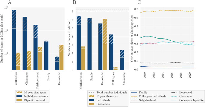
As the network spans an entire population of roughly 7.2 million individuals over multiple years and layers and individuals are by the definition of the layers highly clustered, it contains a substantial number of edges (Fig. 1A). The number of edges varies substantially between layers. For example, households connect only a small set of individuals (4.6 million for a single year), compared to relations formed among colleagues which sum up to 800.6 million for a 10 year time-span (note the log-scale in Fig. 1A). The cause for the increased efficiency of the bipartite view for various computations becomes apparent when considering the difference of the number of edges between the two views. By connecting individuals via shared containers, the bipartite view drastically decreases the number of edges, especially for the large colleague and classmate layer for which the bipartite view only contains a fraction of the number of edges of the individual-centered view. This reduction goes up to 98% when comparing the classmate layer with a 10 year time-span of the bipartite to the individual-centered view. The only exception here is the household layer because in the bipartite view single households also have a single edge to an individual container. The diminished number of edges in the bipartite view is accompanied by a relatively small increase in the total number of nodes caused by the addition of the container nodes (Fig. 1B—note the linear scale). This results in relevant efficiency gains for most graph algorithms, for example shortest paths. Consider the Dijkstra algorithm with a time complexity that is at best (mathscr {O}((Vlog V) + E))²⁹ where the number of nodes (vertices) is denoted by V and the number of edges by E. As in the bipartite view the decrease in the number of edges is much larger compared to the increase in the number of vertices for all time-spans and layers except households, using the bipartite view yields a substantial efficiency gain. Moreover, the bipartite view captures more information than the individual-centered, unipartite one. To illustrate this, consider an example in the colleague layer with multiple years time-span. Due to the possibility of individuals having worked at multiple workplaces over the time span of interest, we cannot infer from three neighboring nodes (a, b, and c) whether they are connected via the same or three separated workplaces where the first workplace connects nodes a and b, the second nodes b and c, and the third nodes a and c. Therefore, the bipartite view cannot be reconstructed from the unipartite projection^17,21. Finally, apart from the computational and conceptual advantages described above, the bipartite view also allows researchers to create their own edge definitions.

Next to the number of depicted relations, the layers also vary in their coverage of the total population, i.e., the number of unique nodes (Fig. 1B). Neighborhood, family, and household information exists for a large share of the overall population, as they are independent of age in contrast to colleagues and classmate relations. The introduction of time-span leads to an increase of the number of nodes because individuals who have graduated (classmate layer), moved to another country (neighborhood and household layer), retired (colleagues layer), or have deceased in the past are also included.

Size and temporal stability of the network. (A) shows the total number of edges per layer for a single year (i.e., 2021) and a 10 year time-span for the bipartite and the individual-centered representation of the network (log scale). (B) shows the total number of nodes per layer for a single year and 10 year time-span for the individual-centered and the bipartite representation of the network. Note that the family layer does not include bipartite nodes and that there are too little classmate container layers to be visible. A table with the number of edges can also be found in Appendix E, Table 1. (C) depicts the year-over-year share of changing edges, i.e., the number of edges in 1 year that also exist in the next year relative to the total number of edges.

Full size image

Overlaps and evolution of network layers

The increase in the number of edges in time-span depends not only on the number of nodes but also reveals information of the stability of the underlying relation. Figure 1C depicts the year-over-year share of changing edges for different layers. While a single digit percentage of family and household relations change every year, neighborhood, job- and participation in educational programs fluctuate more frequently. There is also a substantial difference for the colleagues between the views because of the noise added by the sampling in the individual-centered view.

In our multiplex network, the share of overlapping edges between layers reveals how much additional information each layer provides³⁰. Moreover, it can be argued that overlapping edges can indicate tie-strength as individuals sharing multiple foci points are more likely to also have realized interactions. Figure 2 shows the share of overlapping edges between layers, with the y-axis denoting the layers for a single year and the x-axis depicting the layers with the indicated time-span. The heatmap is not symmetric as the baseline for the share is the layer on the y-axis. We observe relatively large overlaps between the household, neighborhood, and family layer, which are partly explained by the definition of the layers, as the household layer is defined as a family-like structure, and neighbors with the same address can become households when they meet one of the household criteria (e.g., become parents). The overlaps for a single year are similar in magnitude to those in the Dutch administrative network¹³. More relevant are the relatively small but in time-span increasing overlaps between all other layers. For example, we can see how workplaces have been a relevant matching foci for future households: 5.1% of all household edges have also been an edge in the colleague layer over the previous 10 years. Overall, the small share of overlapping edges underlines how each layer captures a unique aspect of the social sphere.

Edge overlap with varying time-span. Share of overlapping edges between reference layer (y-axis) and comparison layer (x-axis). The reference layer is measured for the year 2021 for all the plots. The comparison layer includes a time-span of 0, 5, or 10 years before 2021. The overlapping share is computed as the number of overlapping edges divided by the total number of edges of the reference layer. In (A), the comparison layer includes no time-span, in (B) a 5-year time-span, and in (C) a 10 year time-span.

Full size image

Node degree distribution

The number of connections of a node is an important indicator of a node’s centrality and relevance. Figure 3 depicts three different views on the degree distribution. Panel 3A shows the kernel density estimation of the degree distribution depending on layer and time-span. The number of connections naturally vary between layer-types, also becoming apparent by the use of the log-scale on the x-axis. While, e.g., in the household layer 90% of individuals are connected to five or less other individuals for a 10 year time-span, this number is 5915 for connections via the colleague layer. As increasing the time-span adds additional relations, the degree distributions shift upwards for all layers with respectable variation between the family or household and the neighborhood, colleagues or classmate layer. As observed in many other real-world social and artificial networks, the node degrees are highly unequally distributed. Panel 3B highlights this by depicting the share of nodes ordered by their degree on the x-axis and the share of the accumulated total degree on the y-axis. Put differently, the bottom x-percentage of the degree distribution account for the corresponding y-percentage of total degree and if all nodes would have the same degree, the line would equal the bisecting, dotted line. While we observe inequality in degree in all layers, these are most substantial in the colleague and classmate layer, in which the top 20% of the distribution accounts for roughly half of all connections. Panel 3C underlines that the distributions are heavy-tailed when stacking up the layers to a single network: a large share of the overall distribution is accounted for by relatively few, highly central nodes. With this concentration of degree our network resembles results that are also found in other realized⁸ or administrative¹³ social networks.

Degree distribution. (A) shows the kernel density estimation for the degree distribution for single year (i.e., 2021), 5 and 10 year time-span (log scale). (B) depicts the Lorenz-curve (cumulative share of degrees for lower x-% of nodes) by layer. (C) shows the degree distribution (log-scale) for stacked layers.

Full size image

Next, we analyze whether the fat-tailed, stacked degree distribution is driven by single layers or whether individuals having a large number of connections in one layer directly implies that those individuals also have comparably more connections in other layers. Figure 4 depicts the interlayer degree correlation for different time-spans. We observe no substantive correlations of degree for almost all layers considering a single year time-span. This resembles the results found in the Dutch administrative network^13,16. However, the inter-layer degree correlation increases substantially in magnitude with rising time-span across layers. The correlation is especially pronounced between the family, household, and neighborhood layers. The increase in correlation coefficients over time-span indicates that more well-connected nodes on some layer are more likely to have more edges on other layers and that this effect accumulates over time.

As an illustration of how the network data can be merged with other register data to investigate relevant research questions, we also investigate how the degree as an indicator for social opportunities reflects life outcomes. Figure 5 shows how the average degree sorts closely by the income for a given age. The degree-differences by income are especially pronounced for persons in the middle of their life between ages 25 and 60 and when taking past connections into account (Fig. 5B). This corresponds to the results found in the Dutch administrative network¹³. It has also been suggested in the literature that women have a lower average degree than men, leading to labor market differences³¹. Figure 5C, D show that in our network women indeed have a lower average degree when conditioning on age for most of the working life cycle. However, upon reaching pension age this relationship reverses, although only slightly. While neither of these findings imply any causality, it underlines how closely the network’s centrality and socioeconomic trajectories interrelate. Additionally, it demonstrates the potential of integrating further individual-level data from registries into the network.

Inter-layer degree correlation. Pearson correlation between node’s degree for varying layers and time-span. The time-span applies to the layers on both the x- and y-axis. (A) shows the correlation with no time-span, (B) with time-span of 5 years and (C) with time-span 10 years.

Full size image

Relation of individual degree and income or sex over the working life cycle. Average degree distribution conditional on age and income (A and B) or age and sex (C and D). The plot is based on 2021 data. (A) and (C) contain a single year time-span and (B) and (D) a 10 year time-span.

Full size image

Spatial distribution

A key property of many of our networks’ foci is that they are attributed to specific physical spaces. The household and neighborhood layer are explicitly defined via the home address and the the classmate and colleague layer are associated with specific schools or workplaces. Our network thus can add to research questions in the realm of spatial, social networks. The rich literature in spatial networks investigates the relation between nodes’ spatial distribution and network structure^32,33 and how this relationship affects outcomes such as the transmission of infectious diseases³⁴ or the prevalence of crime³⁵. Figure 6 depicts two descriptive plots on the relation between spatial distance—measured as the euclidean distance between homes—and network connectivity. Panel 6A depicts an estimate on the probability of nodes within a varying spatial radius to also have an edge in the network. Both the definition of the neighborhood and the household layer imply that spatially close-by nodes are likely to also have an edge between them. The probability of being connected in the network starkly decreases in spatial distance, from 26.1% in a radius of 100 meters to 1.1% in a radius of 1 kilometer. Similarly, the distribution of the spatial distance between nodes that are connected in the network (Fig. 6B) is strongly right-skewed. These results highlight the close relation between spatial distances and network connectivity, which are both driven by the definition of the layers and social-spatial clustering. The plots showcasing how the network’s spatial attributes can be utilized should encourage further research to disentangle these two effects.

Spatial distribution and edges. (A) shows the number of edges relative to the total number of possible edges an individual has in a given distance from their home location. The plot shows data for a random sample of 1000 nodes. (B) depicts the distribution of spatial distances between homes of 100,000 random neighboring nodes in the network. The distance measure in both plots is euclidean distance.

Full size image

Higher-order clustering

Because relations form via shared foci, most network layers are highly clustered by design. Therefore investigation of clustering only begins to reveal socially relevant information when considering connections spanning multiple years or considering multiple layers at the same time. Beyond the tendency of nodes to form triangles, the importance of higher-order structures in complex (social) networks has been emphasized in recent literature^36,37,38. This also includes the investigation of higher-order clustering coefficients³⁸. The (ell)-order clustering coefficient (C_{ell }) measures the probability of an (ell)-sized cliques and a randomly drawn adjacent node to form an (ell +1) clique. For (ell =2) the higher-order clustering coefficient simply equals the canonical clustering coefficient. To give an example from our network, consider the classmate layer and the third-order clustering coefficient. The local clustering coefficient for a person would give the probability that of three of its classmates a randomly drawn further neighboring node would also share that class. It is thus a measure of the relevance of cliques of different sizes. A visualization of the higher-order clustering coefficient can be found in Appendix B.

Figure 7 depicts the distribution for higher-order clustering for cliques of two and three when combining all layers for a single year using the bipartite view. We observe a large share of nodes with almost complete higher-order clustering for both (ell): 7.1% (10.3%) of nodes have a clustering coefficient larger than 0.95 for cliques of size two (three). This means that for at least 95% of all cliques of size (ell) that these nodes are part of, any additional neighboring node is also part of an (ell +1)-sized clique. For (ell =3), the distribution of clustering coefficients shifts right and the average local clustering coefficient increases, going against the observations in multiple artificial and real-world networks³⁸. This result indicates the high relevance of larger highly-clustered groups in our network. It thus underlines how not only the individual layers but also the network of combined layers can be understood as one of foci group affiliation, adding an additional rationale for the bipartite perspective. In Appendix C, we present how we utilized the bipartite structure to efficiently compute the higher-order clustering at scale.

Higher-order network clustering. Density of higher-order local clustering coefficients. (A) shows for cliques of size 2 and (B) for size 3.

Full size image

Shortest paths distributions

The average distance between a node to all other nodes is an important measure for social distance, information transitivity, or disease spreading^1,8,39,40. In large-scale networks, computing distances between nodes becomes increasingly computationally expensive as the complexity for commonly used search algorithms (e.g., the Dijkstra or Johnson algorithm) grows both in the number of nodes and edges^29,41,42. We therefore sample shortest-path length distributions by computing the distances between 1000 nodes chosen uniform at random from the node set to 1000 other nodes chosen in the same fashion, shown in Fig. 9A for different layers and time-spans. Note that we exclude pairs that are located in separate, unconnected components of the network.

Comparing the individual layers, we observe different magnitudes and effects of time-span: The family layers’ average distance hardly changes over time and connects a large fraction of the population. Within the neighborhood, classmate and colleague layers, the addition of past connections decreases the average distance between individuals for larger time-spans due to a higher number of bridges between the locally clustered connected components. Households are relatively stable, small-scale and completely clustered foci. Therefore paths exist only in large samples and all nodes in our sample are unconnected except for a single pair until a 10 year time-span.

For many research questions in social science and beyond, combining multiple layers is important. This is because instead of isolated social foci, researchers are interested in the joint social interaction space, e.g., when attempting to trace where an individual was infected with a virus. The different scales and temporal patterns of average path lengths and the variations in degree suggest that the likelihood that an edge in a given layer represents an actual social interaction is not equal for each layer. Treating node-distances the same for every layer would mean that an individual would have the same distance to a colleague in a workplace with a thousand employees as to their child. Since the meaning and significance of connections between nodes can vary with the research question, it is important to be able to adjust the distances to fit the project at hand project. Previous work has used edge-weights to reduce the effect of joint participation in large-scale events on distances⁴³. Similarly, we propose a rational for adjusting edge-weights between individuals to reflect the distinct nature of the layers as visualized in Fig. 8. This endeavor is conceptually akin to adjusting edge-weights in the construction of backbone networks. However, instead of removing edges based on their significance, we allow weights to differ depending not only on their degree but also the nature of the layer⁴⁴. For the network of combined layers to reflect meaningful distances, we set the distance between individuals as a reference with unit length one. We gauge the other layer’s edge-weights against that. We assume household connections to be the strongest as interactions in households are highly likely to occur frequently. We therefore set the weight of persons to the household container node to 1/6, so that two persons in the same household have distance 1/3. In the bipartite view of the network, neighborhoods are connected to each other via address containers. We set the weight between the address containers to 1/3 so that two individuals living at the exact same address but not forming a household (e.g., roommates in a dorm) have distance 1, thus the same distance as family members. We assume neighbors living at a different address to have a lower interaction likelihood and therefore set the weight between addresses to 1/2 so that neighbors have distance 3/2. Opposite to the above mentioned weight adjustments for the family, household and neighborhood layers, the edge-weights for the colleague and classmate layer are discounted contingent to the degree of the container node. The underlying assumption is that the likelihood of realized interactions at the workplace and in school programs decreases with the number of colleagues or classmates, following the idea of agent-/artifact-degree conditioning in backbone construction⁴⁴. A more detailed description of the weighting for the colleague and classmate layers can be found in Appendix D.

We compute the average distance between a random sample of a thousand individuals to another thousand individuals in this network. The resulting distribution (Fig. 9B) is sharply-peaked with an average distance of 5.6, which aligns with the “six degrees of separation” found in many social networks, e.g., online platforms⁹ or communication networks^8,45. Note that the weights we used are just one suggestion that leads to intuitive lengths. Weights can be easily tailored to domain knowledge for a given research purpose. An analysis of the robustness of the suggested weights can be found in Appendix D.

Bipartite representation and edge weighting scheme. Visualization of the suggested weighting scheme for meaningful distances. Individual nodes are depicted as blue circles and container nodes as yellow squares with the number or sign on the nodes denoting the individuals’ pseudo id for visualization purposes or the abbreviated container type (“C” for classroom, “H” for household, “A” for address, “W” for workplace). The number or sign on the edge indicates the suggested weight. The distances between colleagues and classmates are adjusted to the degree of the container node, i.e., the size of the workplace or class (for details see Appendix D). Note that all of these weights can be customized to the research question at hand using the regnet Python package.

Full size image

Shortest-path lengths. (A) illustrates the distribution of the average shortest path for a sample of 1000 random nodes to another 1000 random nodes for different layers, and time-spans (x-axis and color). The number above the plots indicates the share of unconnected nodes in the sample. (B) shows the distribution of 1 million random distances in the bipartite network with all layers combined. The edge-weights are adjusted to reflect meaningful relationships between the layers.

Full size image

Software and Python package

For the construction of the bipartite view and to compute relevant network metrics, researchers get access to the regnet Python software¹⁸. The package is based on the Python interface for the C library igraph, which is also used to create graphs and compute network metrics for the individual-centered view. More details on the regnet software can be found in Appendix A and the repository¹⁸.

In this paper, we have presented a new, nation-scale network dataset derived from Danish registry data containing relationships for multiple central levels of potential social interactions. Unlike any other published administrative network dataset, this network spans more than a dozen years and is accessible in a dual view—an individual-centered view that only contains individuals and their relations and a bipartite view including container nodes at which individuals cluster. We have shown that the bipartite view is founded in network theory, conceptually plausible because of the high clustering of nodes around shared foci and results in efficiency gains due to the drastically reduced number of edges. Furthermore, we introduce an edge-weighting scheme that makes it possible to connect multiple layers while maintaining plausible distances between individuals. This weighting of edges within the bipartite view is implemented in a comprehensive Python package that is published alongside the dataset. Exploring its central characteristics, the network incorporates insightful yet intuitive social properties. These include the heterogenous, heavy-tailed distribution of degree, a time-span increasing inter-layer degree correlation, small but relevant overlaps between different layers, a strong relation between connectivity in the network and spatial distance, as well as the striking relationship between an individuals’ number of connections and their relative income position within the same age group.

By making the network accessible to the research community, we are confident that this dataset can play a central role in a wide range of fields. One important limitation to consider is that the edges in our network do not describe actual interactions but only increased probability for interaction due to a shared social focus. This limits the possibilities to investigate social dynamics on a micro-level, especially when researchers are only interested in a small subset of nodes or do not have prior knowledge of the nature of the relation they are interested in. However, for many research questions, such as the study of social mobility, examining the relationship between broader network structure and individual-level outcomes is at the core of the inquiry^46,47,48. We believe that our network in combination with individual-level administrative data gives rise to many interesting use cases, further extending existing social science research. In the following, we list just a few examples:

First, research could analyze nation-scale network data over longer time horizons that would enable tracking of social cohesion, e.g., by measuring the connectedness of the social network across time and sorting by individuals’ sociodemographic attributes. Second, research could combine the rich administrative data on individuals’ connections and characteristics with survey data to estimate micro-level relational data^49,50,51. Third, future work should explore the relationship between geospatial features and network structure in more depth to investigate the mediating role of urban planning⁵², the interaction between spatial and social distance for disease spread⁵³, and sociospatial segregation⁵⁴. Fourth, further studies could utilize the bipartite view and additionally attach administrative attributes to the container nodes to investigate the relation of institutional and individual influences on link formation. Finally, new research could use the social measure to understand peer effects and social influence⁵⁶ using accurate individual measures that are often not available to social media companies. The administrative data also allows researchers to establish causal social effects, e.g., externalities in the domains of consumption^56,57, family and health behavior^58,59, political concerns⁵¹.